Note
Click here to download the full example code
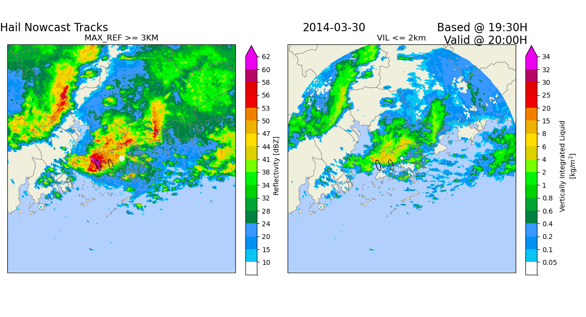
Hail Nowcast (Hong Kong)
This example demonstrates a rule-based hail nowcast for the next 30 minutes, using data from Hong Kong.
Definitions
Import all required modules and methods:
# Python package to allow system command line functions
import os
# Python package to manage warning message
import warnings
# Python package for time calculations
import pandas as pd
# Python package for numerical calculations
import numpy as np
# Python package for xarrays to read and handle netcdf data
import xarray as xr
# Python package for projection
import cartopy.crs as ccrs
# Python package for land/sea features
import cartopy.feature as cfeature
# Python package for reading map shape file
import cartopy.io.shapereader as shpreader
# Python package for creating plots
from matplotlib import pyplot as plt
# Python package for ellipse patches
from matplotlib.patches import Arc
# Python package for colorbars
from matplotlib.colors import BoundaryNorm, ListedColormap

# swirlspy qpf function
from swirlspy.qpf import rover
# swirlspy data parser function
from swirlspy.rad import read_iris_grid, calc_vil
# swirlspy test data source locat utils function
from swirlspy.qpe.utils import timestamps_ending, locate_file
# swirlspy hail labeled and fitted function
from swirlspy.object import get_labeled_frame, fit_ellipse
# swirlspy standardize data function
from swirlspy.utils import standardize_attr, FrameType
# directory constants
from swirlspy.tests.samples import DATA_DIR
from swirlspy.tests.outputs import OUTPUT_DIR

warnings.filterwarnings("ignore")
plt.switch_backend('agg')
Define the working directories:
radar_dir = os.path.abspath(os.path.join(DATA_DIR, 'iris/3d'))
Define the basemap:
# define the plot function
def plot_base(ax: plt.Axes, extents: list, crs: ccrs.Projection):
    # fake the ocean color
    ax.imshow(
        np.tile(np.array([[[178, 208, 254]]], dtype=np.uint8), [2, 2, 1]),
        origin='upper', transform=crs,
        extent=extents, zorder=-1
    )
    # coastline, province and state, color
    ax.add_feature(
        map_with_province, facecolor=cfeature.COLORS['land'],
        edgecolor='none', zorder=0
    )
    # overlay coastline, province and state without color
    ax.add_feature(
        map_with_province, facecolor='none', edgecolor='gray', linewidth=0.5
    )
    ax.set_title('')


# Logging
start_time = pd.Timestamp.now()
Loading radar data
# Specify the basetime
basetime = pd.Timestamp('201403301930')

# Generate timestamps for the current and past 6 minute
# radar scan
timestamps = timestamps_ending(
    basetime,
    duration=pd.Timedelta(6, 'm'),
    exclude_end=False
)

# Locating the files
located_files = []
for timestamp in timestamps:
    located_files.append(locate_file(radar_dir, timestamp))

# Reading the radar data
reflectivity_list = []
for filename in located_files:
    reflectivity = read_iris_grid(filename)
    reflectivity_list.append(reflectivity)

# Standardize reflectivity xarrays
raw_frames = xr.concat(reflectivity_list,
                       dim='time').sortby(['y'], ascending=False)
standardize_attr(raw_frames, frame_type=FrameType.dBZ)

initialising_time = pd.Timestamp.now()
Identify regions of interest for hail
Hail has a chance of occurring when two phenomena co-happen:
The 58 dBZ echo top exceeds 3 km.
The Vertically Integrated Liquid (VIL) up to 2 km is less than 5mm.
# getting radar scan for basetime
reflectivity = raw_frames.sel(time=basetime)

# maximum reflectivity at elevations > 3km
ref_3km = reflectivity.sel(
    height=slice(3000, None)
).max(dim='height', keep_attrs=True)

# 58 dBZ echo top exceeds 3km
cond_1 = ref_3km > 58

# vil up to 2km
vil_2km = calc_vil(reflectivity.sel(height=slice(1000, 2000)))

# VIL up 2km is less than 5mm
cond_2 = vil_2km < 5

# Region of interest for hail
try:
    hail = xr.ufuncs.logical_and(cond_1, cond_2)
except AttributeError:
    # Handle module 'xarray' has no attribute 'ufuncs'
    import numpy as np
    hail = np.logical_and(cond_1, cond_2)
The identified regions are then labeled and fitted with minimum enclosing ellipses.
# label image
# image is binary so any threshold between 0 and 1 works
# define minimum size as 4e6 m^2 or 4 km^2
labeled_hail, uids = get_labeled_frame(hail, 0.5, min_size=4e6)

# fit ellipses to regions of interest
ellipse_list = []
for uid in uids:
    ellipse, _ = fit_ellipse(labeled_hail == uid)
    ellipse_list.append(ellipse)

identify_time = pd.Timestamp.now()
Extrapolation of hail region
First, we obtain the xarray.DataArray to generate the motion field.
In this example, we generate the motion field from two consecutive 3km CAPPI radar scans closest to basetime.
# Select radar data at 3km
frames = raw_frames.sel(height=3000).drop('height')
Obtain the motion field by ROVER
# ROVER
motion = rover(frames)

motion_time = pd.Timestamp.now()
RUNNING 'rover' FOR EXTRAPOLATION.....
Next, we extract the motion vector at the centroid of each ellipse, and calculate the displacement of the ellipse after 30 minutes. Since the distance is expressed in pixels, we need to convert the distance of the motion vector to grid units (in this case, meters).
# getting meters per pixel

area_def = reflectivity.attrs['area_def']
x_d = area_def.pixel_size_x
y_d = area_def.pixel_size_y

# time ratio
# time ratio between nowcast interval and unit time
time_ratio = pd.Timedelta(30, 'm') / pd.Timedelta(6, 'm')

ellipse30_list = []
for ellipse in ellipse_list:
    # getting motion in pixels/6 minutes
    pu = motion[0].sel(x=ellipse['center'][0],
                       y=ellipse['center'][1],
                       method='nearest')
    pv = motion[1].sel(x=ellipse['center'][0],
                       y=ellipse['center'][1],
                       method='nearest')
    # converting to meters / 6 minutes
    u = x_d * pu
    v = y_d * pv
    # get displacement in 30 minutes
    dcenterx = u * time_ratio
    dcentery = v * time_ratio
    # get new position of ellipse after 30 minutes
    x30 = ellipse['center'][0] + dcenterx
    y30 = ellipse['center'][1] + dcentery
    # get new ellipse, only the center is changed
    ellipse30 = ellipse.copy()
    ellipse30['center'] = (x30, y30)

    ellipse30_list.append(ellipse30)


extrapolate_time = pd.Timestamp.now()
Visualisation
# Defining figure
fig = plt.figure(figsize=(12, 6.5))
# number of rows and columns in plot
nrows = 2
ncols = 1
# Defining the crs
crs = area_def.to_cartopy_crs()

# Load the shape of Hong Kong
map_shape_file = os.path.abspath(
    os.path.join(DATA_DIR, 'shape/hk_tms_aeqd.shp')
)

# coastline and province
map_with_province = cfeature.ShapelyFeature(
    list(shpreader.Reader(map_shape_file).geometries()),
    area_def.to_cartopy_crs()
)

# Defining extent
x = labeled_hail.coords['x'].values
y = labeled_hail.coords['y'].values
x_d = x[1] - x[0]
y_d = y[1] - y[0]
extents = [x[0], y[0], x[-1], y[-1]]


# Defining ellipse patches
def gen_patches(lst, ls='-'):
    patch_list = []
    for ellipse in lst:
        patch = Arc(
            ellipse['center'],
            ellipse['b'] * 2,
            ellipse['a'] * 2,
            angle=ellipse['angle'],
            ls=ls
        )
        patch_list.append(patch)
    return patch_list


# 1. Plotting maximum reflectivity above 3km
# Define color scheme
# Defining colour scale and  format.
levels = [
    -32768, 10, 15, 20, 24, 28, 32, 34, 38, 41,
    44, 47, 50, 53, 56, 58, 60, 62
]
cmap = ListedColormap([
    '#FFFFFF00', '#08C5F5', '#0091F3', '#3898FF', '#008243', '#00A433',
    '#00D100', '#01F508', '#77FF00', '#E0D100', '#FFDC01', '#EEB200',
    '#F08100', '#F00101', '#E20200', '#B40466', '#ED02F0'
])

norm = BoundaryNorm(levels, ncolors=cmap.N, clip=True)

ax = fig.add_subplot(ncols, nrows, 1, projection=crs)
plot_base(ax, extents, crs)
ref_3km.where(ref_3km > levels[1]).plot(
    ax=ax,
    cmap=cmap,
    norm=norm,
    extend='max',
    cbar_kwargs={
        'ticks': levels[1:],
        'format': '%.3g',
        'fraction': 0.046,
        'pad': 0.04
    }
)
patches = gen_patches(ellipse_list)
for patch in patches:
    ax.add_patch(patch)
patches = gen_patches(ellipse30_list, ls='--')
for patch in patches:
    ax.add_patch(patch)
ax.set_title('MAX_REF >= 3KM')

# 2. Plotting VIL up to 2km
levels = [
    0, 0.05,
    0.1, 0.2, 0.4, 0.6, 0.8, 1,
    2, 4, 6, 8, 15, 20,
    25, 30, 32, 34
]
cmap = ListedColormap([
    '#FFFFFF', '#08C5F5', '#0091F3', '#3898FF', '#008243', '#00A433',
    '#00D100', '#01F508', '#77FF00', '#E0D100', '#FFDC01', '#EEB200',
    '#F08100', '#F00101', '#E20200', '#B40466', '#ED02F0'
])

norm = BoundaryNorm(levels, ncolors=cmap.N, clip=True)
ax = fig.add_subplot(ncols, nrows, 2, projection=crs)
plot_base(ax, extents, crs)

vil_2km.where(vil_2km > levels[1]).plot(
    cmap=cmap,
    norm=norm,
    ax=ax,
    extend='max',
    cbar_kwargs={
        'ticks': levels[1:],
        'format': '%.3g',
        'fraction': 0.046,
        'pad': 0.04
    }
)
ax.set_title('VIL <= 2km')
patches = gen_patches(ellipse_list)
for patch in patches:
    ax.add_patch(patch)
patches = gen_patches(ellipse30_list, ls='--')
for patch in patches:
    ax.add_patch(patch)

suptitle1 = "Hail Nowcast Tracks"
suptitle2 = basetime.strftime('%Y-%m-%d')
suptitle3 = (f"Based @ {basetime.strftime('%H:%MH')}\n"
             f"Valid @ {(basetime + pd.Timedelta(30, 'm')).strftime('%H:%MH')}")
fig.text(0., 0.93, suptitle1, va='top', ha='left', fontsize=16)
fig.text(0.57, 0.93, suptitle2, va='top', ha='center', fontsize=16)
fig.text(0.90, 0.93, suptitle3, va='top', ha='right', fontsize=16)
plt.tight_layout()
plt.savefig(
    os.path.join(OUTPUT_DIR, "hail.png"),
    dpi=300
)

visualise_time = pd.Timestamp.now()
Checking run time of each component
print(f"Start time: {start_time}")
print(f"Initialising time: {initialising_time}")
print(f"Identify time: {identify_time}")
print(f"Motion field time: {motion_time}")
print(f"Extrapolate time: {extrapolate_time}")
print(f"Visualise time: {visualise_time}")

print(f"Time to initialise: {initialising_time - start_time}")
print(f"Time to identify hail regions: {identify_time - initialising_time}")
print(f"Time to generate motion field: {motion_time - identify_time}")
print(f"Time to extrapolate: {extrapolate_time - motion_time}")
print(f"Time to visualise: {visualise_time - extrapolate_time}")

print(f"Total: {visualise_time - start_time}")
Start time: 2026-04-20 20:22:33.451444
Initialising time: 2026-04-20 20:22:34.425945
Identify time: 2026-04-20 20:22:34.467148
Motion field time: 2026-04-20 20:22:34.542508
Extrapolate time: 2026-04-20 20:22:34.546445
Visualise time: 2026-04-20 20:22:36.363322
Time to initialise: 0 days 00:00:00.974501
Time to identify hail regions: 0 days 00:00:00.041203
Time to generate motion field: 0 days 00:00:00.075360
Time to extrapolate: 0 days 00:00:00.003937
Time to visualise: 0 days 00:00:01.816877
Total: 0 days 00:00:02.911878
Total running time of the script: ( 0 minutes 3.381 seconds)