Note
Click here to download the full example code
Probabilistic Lightning Density Nowcast (Hong Kong)
This example demonstrates how to perform probabilistic lightning nowcast by advecting lightning density, using data from Hong Kong.
Definitions
Import all required modules and methods:
# Python package to allow system command line functions
import os
# Python package to manage warning message
import warnings
# Python package for time calculations
import pandas as pd
# Python package for numerical calculations
import numpy as np
# Python package for xarrays to read and handle netcdf data
import xarray as xr
# Python package for text formatting
import textwrap
# Python package for projection description
import pyproj
from pyresample import get_area_def
# Python package for projection
import cartopy.crs as ccrs
# Python package for land/sea features
import cartopy.feature as cfeature
# Python package for reading map shape file
import cartopy.io.shapereader as shpreader
# Python package for creating plots
from matplotlib import pyplot as plt
# Python package for output grid format
from matplotlib.gridspec import GridSpec
# Python package for colorbars
from matplotlib.colors import BoundaryNorm, ListedColormap
from matplotlib.cm import ScalarMappable

# Python com-swirls package to calculate motion field (rover) and semi-lagrangian advection
from swirlspy.qpf import rover, sla
# swirlspy data parser function
from swirlspy.rad.iris import read_iris_grid
# swirlspy test data source locat utils function
from swirlspy.qpe.utils import timestamps_ending, locate_file
# swirlspy regrid function
from swirlspy.core.resample import grid_resample
# swirlspy lightning function
from swirlspy.obs import Lightning
from swirlspy.ltg.map import gen_ltg_density
# swirlspy standardize data function
from swirlspy.utils import standardize_attr, FrameType
# directory constants
from swirlspy.tests.samples import DATA_DIR
from swirlspy.tests.outputs import OUTPUT_DIR

warnings.filterwarnings("ignore")
plt.switch_backend('agg')
Initialising
Define the target grid:
# Defining target grid
area_id = "hk1980_250km"
description = ("A 1km resolution rectangular grid "
               "centred at HKO and extending to 250 km "
               "in each direction in HK1980 easting/northing coordinates")
proj_id = 'hk1980'
projection = ('+proj=tmerc +lat_0=22.31213333333334 '
              '+lon_0=114.1785555555556 +k=1 +x_0=836694.05 '
              '+y_0=819069.8 +ellps=intl +towgs84=-162.619,-276.959,'
              '-161.764,0.067753,-2.24365,-1.15883,-1.09425 +units=m '
              '+no_defs')

x_size = 500
y_size = 500

area_extent = (587000, 569000, 1087000, 1069000)

area_def = get_area_def(
    area_id, description, proj_id, projection, x_size, y_size, area_extent
)
Define basemap:
# Load the shape of Hong Kong
map_shape_file = os.path.abspath(os.path.join(
    DATA_DIR,
    'shape/hk_hk1980'
))

# coastline and province
map_with_province = cfeature.ShapelyFeature(
    list(shpreader.Reader(map_shape_file).geometries()),
    area_def.to_cartopy_crs()
)


# define the plot function
def plot_base(ax: plt.Axes, extents: list, crs: ccrs.Projection):
    # fake the ocean color
    ax.imshow(
        np.tile(np.array([[[178, 208, 254]]], dtype=np.uint8), [2, 2, 1]),
        origin='upper', transform=crs,
        extent=extents, zorder=-1
    )
    # coastline, province and state, color
    ax.add_feature(
        map_with_province, facecolor=cfeature.COLORS['land'],
        edgecolor='none', zorder=0
    )
    # overlay coastline, province and state without color
    ax.add_feature(
        map_with_province, facecolor='none', edgecolor='gray', linewidth=0.5
    )
    ax.set_title('')
Defining a basetime, nowcast interval and nowcast duration:
basetime = pd.Timestamp('201904201200').floor('min')
basetime_str = basetime.strftime('%Y%m%d%H%M')
nowcast_interval = pd.Timedelta(30, 'm')
nowcast_duration = pd.Timedelta(2, 'h')
Loading Lightning and Radar Data
Extract Lightning Location Information System (LLIS) files to read.
# The interval between LLIS files
llis_file_interval = pd.Timedelta(1, 'm')

# Finding the string representation
# of timestamps marking the relevant LLIS files
timestamps = timestamps_ending(
    basetime,
    duration=nowcast_interval,
    interval=llis_file_interval,
    format='%Y%m%d%H%M'
)

# Locating files
llis_dir = os.path.join(DATA_DIR, 'llis')

located_files = []
for timestamp in timestamps:
    located_file = locate_file(llis_dir, timestamp)
    located_files.append(located_file)
    if located_file is not None:
        print(f"LLIS file for {timestamp} has been located")
LLIS file for 201904201130 has been located
LLIS file for 201904201131 has been located
LLIS file for 201904201132 has been located
LLIS file for 201904201133 has been located
LLIS file for 201904201134 has been located
LLIS file for 201904201135 has been located
LLIS file for 201904201136 has been located
LLIS file for 201904201137 has been located
LLIS file for 201904201138 has been located
LLIS file for 201904201139 has been located
LLIS file for 201904201140 has been located
LLIS file for 201904201141 has been located
LLIS file for 201904201142 has been located
LLIS file for 201904201143 has been located
LLIS file for 201904201144 has been located
LLIS file for 201904201145 has been located
LLIS file for 201904201146 has been located
LLIS file for 201904201147 has been located
LLIS file for 201904201148 has been located
LLIS file for 201904201149 has been located
LLIS file for 201904201150 has been located
LLIS file for 201904201151 has been located
LLIS file for 201904201152 has been located
LLIS file for 201904201153 has been located
LLIS file for 201904201154 has been located
LLIS file for 201904201155 has been located
LLIS file for 201904201156 has been located
LLIS file for 201904201157 has been located
LLIS file for 201904201158 has been located
LLIS file for 201904201159 has been located
Read data from files into Lightning objects.
# Initialising Lightning objects
# Coordinates are geodetic
ltg_object_geodetic = Lightning(
    located_files,
    'geodetic',
    basetime - nowcast_interval,
    basetime
)
Locating IRIS REF radar files needed to generate motion field. The IRIS REF files are marked by start time.
# The interval between the radar files
rad_interval = pd.Timedelta(6, 'm')

# Finding the string representation
# of the timestamps
# marking the required files
# In this case, the most recent radar files
# separated by `nowcast_interval` is required

rad_timestamps = timestamps_ending(
    basetime,
    duration=nowcast_interval + rad_interval,
    interval=rad_interval
)

rad_timestamps = [rad_timestamps[0], rad_timestamps[-1]]

rad_dir = os.path.join(DATA_DIR, 'iris')
located_rad_files = []
for timestamp in rad_timestamps:
    located_file = locate_file(rad_dir, timestamp)
    located_rad_files.append(located_file)
    if located_file is not None:
        print(f"IRIS REF file for {timestamp} has been located")
IRIS REF file for 1904201124 has been located
IRIS REF file for 1904201154 has been located
Read from iris radar files using read_iris_grid(). The data is in the Azimuthal Equidistant Projection.
reflec_unproj_list = []
for file in located_rad_files:
    reflec = read_iris_grid(file)
    reflec_unproj_list.append(reflec)
Data Reprojection
Since the coordinates of the Lightning objects are geodetic, a conversion from geodetic coordinates to that of the user-defined projection system is required. This can be achieved by swirlspy.obs.Lightning.reproject()
# pyproj representation of the map projection of the input data
inProj = pyproj.Proj(init='epsg:4326')
# pyproj representation of the intended map projection
outProj = pyproj.Proj(area_def.proj_str)

# reproject
ltg_object = ltg_object_geodetic.reproject(inProj, outProj, 'HK1980')
Radar data also needs to be reprojected from Azimuthal Equidistant to HK1980. This is achieved by the swirlspy.core.resample function. Following reprojection, the individual xarray.DataArrays can be concatenated to a single xarray.DataArrays.
reflec_list = []
for z in reflec_unproj_list:
    reflec = grid_resample(
        z,
        z.attrs['area_def'],
        area_def,
        coord_label=['easting', 'northing']
    )
    reflec_list.append(reflec)

reflectivity = xr.concat(reflec_list, dim='time')
standardize_attr(reflectivity, frame_type=FrameType.dBZ)

print(reflectivity)
<xarray.DataArray (time: 2, northing: 500, easting: 500)> Size: 4MB
array([[[nan, nan, nan, ..., nan, nan, nan],
        [nan, nan, nan, ..., nan, nan, nan],
        [nan, nan, nan, ..., nan, nan, nan],
        ...,
        [nan, nan, nan, ..., nan, nan, nan],
        [nan, nan, nan, ..., nan, nan, nan],
        [nan, nan, nan, ..., nan, nan, nan]],

       [[nan, nan, nan, ..., nan, nan, nan],
        [nan, nan, nan, ..., nan, nan, nan],
        [nan, nan, nan, ..., nan, nan, nan],
        ...,
        [nan, nan, nan, ..., nan, nan, nan],
        [nan, nan, nan, ..., nan, nan, nan],
        [nan, nan, nan, ..., nan, nan, nan]]])
Coordinates:
  * northing  (northing) float64 4kB 1.068e+06 1.068e+06 ... 5.705e+05 5.695e+05
  * easting   (easting) float64 4kB 5.875e+05 5.885e+05 ... 1.086e+06 1.086e+06
  * time      (time) datetime64[ns] 16B 2019-04-20T11:24:00 2019-04-20T11:54:00
Attributes:
    long_name:     Reflectivity
    units:         dBZ
    projection:    hk1980
    site:          (114.12333341315389, 22.41166664287448, 580)
    radar_height:  8
    area_def:      Area ID: hk1980_250km\nDescription: A 1km resolution recta...
    proj_site:     (830755.3393923986, 830262.1449904075)
    step_size:     0 days 00:30:00
    zero_value:    nan
    frame_type:    FrameType.dBZ
Generating lightning density field
Generate a lightning density field.
Count the number of lightning strikes in a circular search area of 8km surrounding a pixel over the past 30 minutes. Do this for all the pixels.
This value is then spatially and temporally averaged to give a lightning density, an indicator of lightning activity given as the number of strikes/km2/hr.
# Obtaining lightning density from lightning objects
ltg_density = gen_ltg_density(
    ltg_object,
    area_def,
    ltg_object.start_time,
    ltg_object.end_time,
    tolerance=8000,
    coord_label=['easting', 'northing']
)

print(ltg_density)

# Duplicating ltg_density along the time dimension
# so that it can be advected.
ltg_density1 = ltg_density.copy()
ltg_density1.coords['time'] = [basetime - nowcast_interval]
ltg_density_concat = xr.concat(
    [ltg_density1, ltg_density],
    dim='time'
)
# Identifying zero value
ltg_density_concat.attrs['zero_value'] = np.nan
<xarray.DataArray (time: 1, northing: 500, easting: 500)> Size: 2MB
array([[[0., 0., 0., ..., 0., 0., 0.],
        [0., 0., 0., ..., 0., 0., 0.],
        [0., 0., 0., ..., 0., 0., 0.],
        ...,
        [0., 0., 0., ..., 0., 0., 0.],
        [0., 0., 0., ..., 0., 0., 0.],
        [0., 0., 0., ..., 0., 0., 0.]]])
Coordinates:
  * time      (time) datetime64[ns] 8B 2019-04-20T12:00:00
  * northing  (northing) float64 4kB 1.068e+06 1.068e+06 ... 5.705e+05 5.695e+05
  * easting   (easting) float64 4kB 5.875e+05 5.885e+05 ... 1.086e+06 1.086e+06
Attributes:
    long_name:  Lightning density
    units:      strikes/$km^2$/h
Generating motion fields and extrapolating
Generate motion field using ROVER.
Extrapolate lightning density using the motion field by Semi-Lagrangian Advection.
Repeat using different parameters to form an ensemble.
# Different ROVER parameters
params = pd.DataFrame()
params['smallest_scale'] = [1, 1, 1, 2]
params['largest_scale'] = [7, 7, 7, 7]
params['rho'] = [9, 9, 9, 9]
params['alpha'] = [2000, 2000, 10000, 2000]
params['sigma'] = [1.5, 2.5, 1.5, 2.5]
params['tracking_interval'] = [30, 30, 30, 30]

xtrp_frames = []
for i in range(len(params)):
    # Generating motion field using ROVER
    motion = rover(
        reflectivity,
        start_level=params['smallest_scale'][i],
        max_level=params['largest_scale'][i],
        rho=params['rho'][i],
        alpha=params['alpha'][i],
        sigma=params['sigma'][i]
    )
    # SLA
    steps = int(nowcast_duration.total_seconds()
                // nowcast_interval.total_seconds())
    ltg_density_xtrp = sla(ltg_density_concat, motion, nowcast_steps=steps)
    xtrp_frames.append(ltg_density_xtrp)


# Create coordinates for `ensemble` dimension
ens_coords = ["Member-{:02}".format(i) for i in range(len(xtrp_frames))]

# Concat ltg_frames along the ensemble dimension
ltg_frames = xr.concat(xtrp_frames, pd.Index(ens_coords, name='ensemble'))

print(ltg_frames)
RUNNING 'rover' FOR EXTRAPOLATION.....
RUNNING 'rover' FOR EXTRAPOLATION.....
RUNNING 'rover' FOR EXTRAPOLATION.....
RUNNING 'rover' FOR EXTRAPOLATION.....
<xarray.DataArray (ensemble: 4, time: 5, northing: 500, easting: 500)> Size: 40MB
array([[[[ 0.,  0.,  0., ...,  0.,  0.,  0.],
         [ 0.,  0.,  0., ...,  0.,  0.,  0.],
         [ 0.,  0.,  0., ...,  0.,  0.,  0.],
         ...,
         [ 0.,  0.,  0., ...,  0.,  0.,  0.],
         [ 0.,  0.,  0., ...,  0.,  0.,  0.],
         [ 0.,  0.,  0., ...,  0.,  0.,  0.]],

        [[nan, nan, nan, ..., nan, nan, nan],
         [nan, nan, nan, ..., nan, nan, nan],
         [nan, nan, nan, ..., nan, nan, nan],
         ...,
         [nan, nan, nan, ..., nan, nan, nan],
         [nan, nan, nan, ..., nan, nan, nan],
         [nan, nan, nan, ..., nan, nan, nan]],

        [[nan, nan, nan, ..., nan, nan, nan],
         [nan, nan, nan, ..., nan, nan, nan],
         [nan, nan, nan, ..., nan, nan, nan],
         ...,
...
         ...,
         [nan, nan, nan, ...,  0., nan, nan],
         [nan, nan, nan, ..., nan, nan, nan],
         [nan, nan, nan, ..., nan, nan, nan]],

        [[nan, nan, nan, ..., nan, nan, nan],
         [nan, nan, nan, ..., nan, nan, nan],
         [nan, nan, nan, ..., nan, nan, nan],
         ...,
         [nan, nan, nan, ...,  0., nan, nan],
         [nan, nan, nan, ..., nan, nan, nan],
         [nan, nan, nan, ..., nan, nan, nan]],

        [[nan, nan, nan, ..., nan, nan, nan],
         [nan, nan, nan, ..., nan, nan, nan],
         [nan, nan, nan, ..., nan, nan, nan],
         ...,
         [nan, nan, nan, ...,  0., nan, nan],
         [nan, nan, nan, ..., nan, nan, nan],
         [nan, nan, nan, ..., nan, nan, nan]]]])
Coordinates:
  * time      (time) datetime64[ns] 40B 2019-04-20T12:00:00 ... 2019-04-20T14...
  * northing  (northing) float64 4kB 1.068e+06 1.068e+06 ... 5.705e+05 5.695e+05
  * easting   (easting) float64 4kB 5.875e+05 5.885e+05 ... 1.086e+06 1.086e+06
  * ensemble  (ensemble) object 32B 'Member-00' 'Member-01' ... 'Member-03'
Attributes:
    long_name:   Lightning density
    units:       strikes/$km^2$/h
    zero_value:  nan
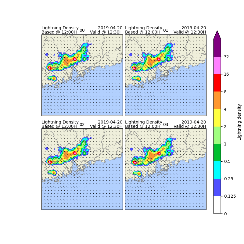
Now, let us visualise the extrapolated lightning density fields for the next 30 minutes.
levels = [
    0, 0.125, 0.25, 0.5, 1,
    2, 4, 8, 16, 32, 999
]
cmap = ListedColormap([
    '#FFFFFF', '#5050FF', '#00FFFF', '#00C030', '#A0FF80',
    '#FFFF40', '#FF9830', '#FF0000', '#FF80FF', '#800080'
])

norm = BoundaryNorm(levels, ncolors=cmap.N, clip=True)

mappable = ScalarMappable(cmap=cmap, norm=norm)
mappable.set_array([])

# Defining the crs
crs = area_def.to_cartopy_crs()

# Defining area
x = ltg_frames.coords['easting'].values
y = ltg_frames.coords['northing'].values
extents = [
    np.min(x), np.max(x),
    np.min(y), np.max(y)
]

qx = motion.coords['easting'].values[::20]
qy = motion.coords['northing'].values[::20]
qu = motion.values[0, ::20, ::20]
qv = motion.values[1, ::20, ::20]

fig = plt.figure(figsize=(8, 8), frameon=False)
gs = GridSpec(
    2, 2, figure=fig, wspace=0.03, hspace=-0.25, top=0.95,
    bottom=0.05, left=0.17, right=0.845
)

# The time to visualise
vis_time = basetime + nowcast_interval

for i, mem in enumerate(ltg_frames.ensemble.values):
    row = i // 2
    col = i % 2
    ax = fig.add_subplot(gs[row, col], projection=crs)

    # plot base map
    plot_base(ax, extents, crs)

    # plot lightning
    frame = ltg_frames.sel(ensemble=mem, time=vis_time)
    frame.where(frame > levels[1]).plot(
        cmap=cmap,
        norm=norm,
        add_colorbar=False
    )

    # plot motion vector
    ax.quiver(
        qx, qy, qu, qv, pivot='mid'
    )

    ax.set_title(mem.split("-")[1], fontsize=10)

    ax.text(
        extents[0],
        extents[3],
        textwrap.dedent(
            """
            Lightning Density
            Based @ {baseTime}
            """
        ).format(
            baseTime=basetime.strftime('%H:%MH')
        ).strip(),
        fontsize=10,
        va='bottom',
        ha='left',
        linespacing=1
    )
    ax.text(
        extents[1],
        extents[3],
        textwrap.dedent(
            """
            {validDate}
            Valid @ {validTime}
            """
        ).format(
            validDate=basetime.strftime('%Y-%m-%d'),
            validTime=vis_time.strftime('%H:%MH')
        ).strip(),
        fontsize=10,
        va='bottom',
        ha='right',
        linespacing=1
    )

cbar_ax = fig.add_axes([0.875, 0.125, 0.03, 0.75])
cbar = fig.colorbar(
    mappable, cax=cbar_ax, ticks=levels[:-1], extend='max', format='%.3g')
cbar.ax.set_ylabel(ltg_frames.attrs['long_name'], rotation=90)

fig.savefig(
    os.path.join(OUTPUT_DIR, "ltg-hk.png"),
    bbox_inches='tight'
)
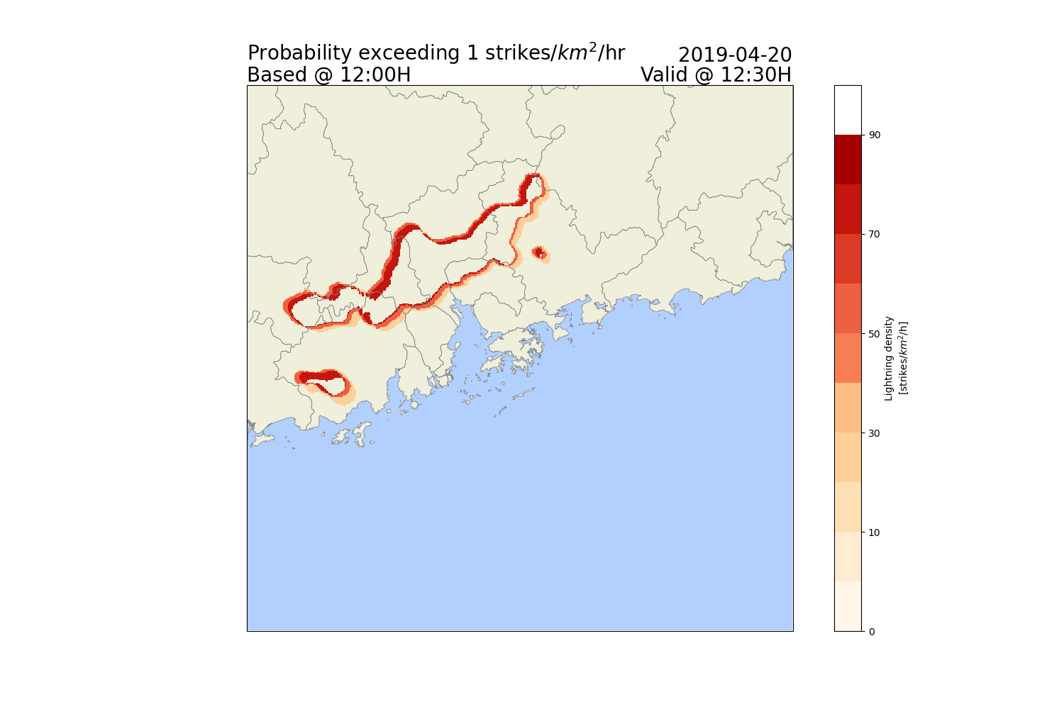
Deriving lightning probabilities
# Finally, it is possible to derive
# the probability of lightning exceeding threshold from our ensemble forecast.
#

# Compute exceedance probabililities for a 1 strikes/km^2/h threshold
P = (ltg_frames > 1).sum(dim='ensemble') / len(ltg_frames.ensemble) * 100

# Define cmap, norm
levels = [
    0, 5, 10, 20, 30, 40, 50, 60, 70, 80, 90, 100
]
cmap = plt.get_cmap("OrRd", len(levels))
norm = BoundaryNorm(levels, ncolors=cmap.N, clip=True)

# Plotting the Exceedance Probability for the first 30 minutes nowcast
fig = plt.figure(figsize=(15, 10))
ax = plt.axes(projection=area_def.to_cartopy_crs())

plot_base(ax, extents, area_def.to_cartopy_crs())

P.where(P > levels[0]).sel(time=vis_time).plot(
    cmap=cmap,
    norm=norm
)

ax.text(
    extents[0],
    extents[3],
    textwrap.dedent(
        """
        Probability exceeding 1 strikes/$km^2$/hr
        Based @ {baseTime}
        """
    ).format(
        baseTime=basetime.strftime('%H:%MH')
    ).strip(),
    fontsize=20,
    va='bottom',
    ha='left',
    linespacing=1
)
ax.text(
    extents[1],
    extents[3],
    textwrap.dedent(
        """
        {validDate}
        Valid @ {validTime}
        """
    ).format(
        validDate=basetime.strftime('%Y-%m-%d'),
        validTime=vis_time.strftime('%H:%MH')
    ).strip(),
    fontsize=20,
    va='bottom',
    ha='right',
    linespacing=1
)

ax.set_title("")

fig.savefig(
    os.path.join(OUTPUT_DIR, "ltg-hk-p.png"),
    bbox_inches='tight'
)
Total running time of the script: ( 0 minutes 36.005 seconds)