QPF (Malaysia)

This example demonstrates how to perform operational deterministic QPF up to three hours using national radar data.

Definitions

Import all required modules and methods:

# Python package to allow system command line functions
import os
# Python package to manage warning message
import warnings
# Python package for timestamp
import pandas as pd
# Python package for xarrays to read and handle netcdf data
import xarray as xr
# Python package for numerical calculations
import numpy as np
# Python package for reading map shape file
import cartopy.io.shapereader as shpreader
# Python package for land/sea features
import cartopy.feature as cfeature
# Python package for projection
import cartopy.crs as ccrs
# Python package for creating plots
from matplotlib import pyplot as plt
# Python package for output import grid
from matplotlib.gridspec import GridSpec
# Python package for colorbars
from matplotlib.colors import BoundaryNorm, ListedColormap
# Python package for scalar data to RGBA mapping
from matplotlib.cm import ScalarMappable

# Python com-swirls package to standardize attributes
from swirlspy.utils import standardize_attr, FrameType
# Python com-swirls package to calculate motion field (rover) and semi-lagrangian advection
from swirlspy.qpf import rover, sla
# directory constants
from swirlspy.tests.samples import DATA_DIR
from swirlspy.tests.outputs import OUTPUT_DIR

warnings.filterwarnings("ignore")

start_time = pd.Timestamp.now()

Initialising

This section demonstrates extracting radar reflectivity data.

Step 1: Define your input data directory and output directory

# Supply the directory of radar and nwp data
data_dir = os.path.abspath(
    os.path.join(DATA_DIR, 'netcdf_ms')
)

Step 2: Define a basetime

# Supply basetime
basetime = pd.Timestamp('201908090900')

Step 3: Read data files from the radar data using xarray()

# Radar data listed from the basetime[0] --> 3 hours before the basetime[17] (descending time)
interval = 10             # Interval of radar data
radar_datas = []
for i in range(0, 2):
    t = basetime - pd.Timedelta(minutes=i * interval)
    # Radar data nomenclature
    filename = os.path.join(
        data_dir,
        t.strftime("radar_d03_%Y-%m-%d_%H_%M_00.rapids.nc")
    )
    reflec = xr.open_dataset(filename)
    radar_datas.append(reflec)

# Concatenate list by time
reflec_concat = xr.concat(radar_datas, dim='time')

# Extracting the radar data: The radar dBZ variable is named 'Zradar', therefore, we extract 'Zradar'
radar = reflec_concat['Zradar']

# Reversing such that time goes from earliest to latest; 3 hours before basetime[0] --> basetime[17]
radar = radar.sortby('time', ascending=True)

# Filtering
radar = radar.where(radar > 15, np.nan)

initialising_time = pd.Timestamp.now()

Nowcast (SWIRLS-Radar-Advection)

The swirls radar advection was performed using the observed radar data Firstly, some attributes necessary for com-swirls input variable is added Secondly, rover function is invoked to compute the motion field Thirdly, semi-lagrangian advection is performed to advect the radar data using the rover motion field

# Adding in some attributes that is step_size <10 mins in pandas.Timedelta>, zero_value <9999.> frame_type <FrameType.dBZ>
standardize_attr(radar, frame_type=FrameType.dBZ, zero_value=np.nan)

# Rover motion field computation
motion = rover(radar)
rover_time = pd.Timestamp.now()

# Semi-Lagrangian Advection
swirls = sla(radar, motion, 18)  # Radar time goes from earliest to latest
sla_time = pd.Timestamp.now()

RUNNING 'rover' FOR EXTRAPOLATION.....

Plotting result

Step 1: Defining the dBZ levels, colorbar parameters and projection

# levels of colorbar (dBZ)
levels = [-32768, 10, 15, 20, 24, 28, 32, 34, 38, 41, 44,
          47, 50, 53, 56, 58, 60, 62]
# hko colormap for dBZ at each levels
cmap = ListedColormap([
    '#FFFFFF', '#08C5F5', '#0091F3', '#3898FF', '#008243', '#00A433',
    '#00D100', '#01F508', '#77FF00', '#E0D100', '#FFDC01', '#EEB200',
    '#F08100', '#F00101', '#E20200', '#B40466', '#ED02F0'
])
# boundary
norm = BoundaryNorm(levels, ncolors=cmap.N, clip=True)
# scalar data to RGBA mapping
scalar_map = ScalarMappable(cmap=cmap, norm=norm)
scalar_map.set_array([])
# Defining plot parameters
map_shape_file = os.path.abspath(os.path.join(
    DATA_DIR,
    'shape/se_asia'
))
# coastline and province
se_asia = cfeature.ShapelyFeature(
    list(shpreader.Reader(map_shape_file).geometries()),
    ccrs.PlateCarree()
)
# output area
extents = [99, 120, 0.5, 7.25]

# base_map plotting function
def plot_base(ax: plt.Axes):
    ax.set_extent(extents, crs=ccrs.PlateCarree())

    # fake the ocean color
    ax.imshow(np.tile(np.array([[[178, 208, 254]]],
                               dtype=np.uint8), [2, 2, 1]),
              origin='upper',
              transform=ccrs.PlateCarree(),
              extent=[-180, 180, -180, 180],
              zorder=-1)
    # coastline, state, color
    ax.add_feature(se_asia,
                   facecolor=cfeature.COLORS['land'], edgecolor='none', zorder=0)
    # overlay coastline, state without color
    ax.add_feature(se_asia, facecolor='none',
                   edgecolor='gray', linewidth=0.5)

    ax.set_title('')

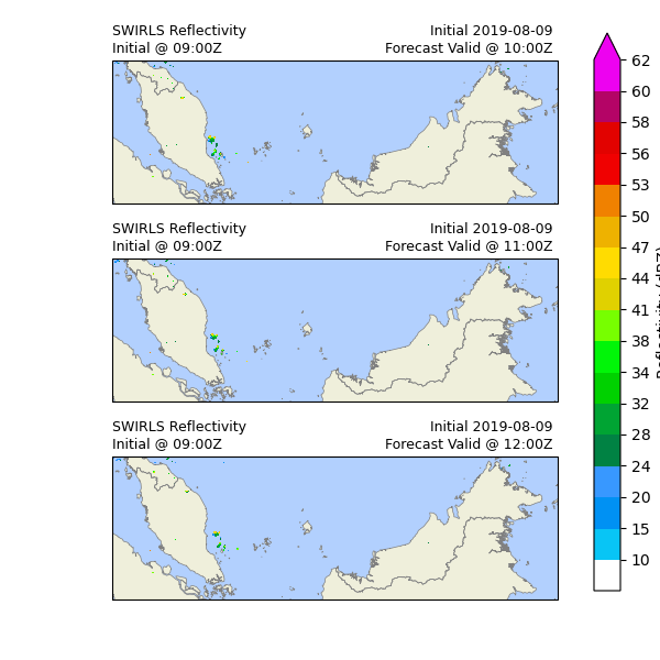
Step 2: Plotting the swirls-radar-advection, nwp-bias-corrected, blended 3 hours ahead

fig: plt.Figure = plt.figure(
    figsize=(5 + 1, 3 * 2),
    frameon=False
)
gs = GridSpec(
    3, 1, figure=fig,
    wspace=0.03, hspace=0, top=0.95, bottom=0.05, left=0.17, right=0.845
)

for row in range(3):
    time_index = (row + 1) * 6
    timelabel = basetime + pd.Timedelta(interval * (time_index), 'm')

    ax: plt.Axes = fig.add_subplot(
        gs[row, 0],
        projection=ccrs.PlateCarree()
    )
    z = swirls[time_index].values
    lats = swirls[time_index].latitude
    lons = swirls[time_index].longitude
    title = 'SWIRLS Reflectivity'

    # plot base map
    plot_base(ax)

    # plot reflectivity
    ax.contourf(
        lons, lats, z, 60,
        transform=ccrs.PlateCarree(),
        cmap=cmap, norm=norm, levels=levels
    )

    ax.set_title(
        f"{title}\n" +
        f"Initial @ {basetime.strftime('%H:%MZ')}",
        loc='left', fontsize=9
    )
    ax.set_title('')
    ax.set_title(
        f"Initial {basetime.strftime('%Y-%m-%d')} \n" +
        f"Forecast Valid @ {timelabel.strftime('%H:%MZ')} ",
        loc='right', fontsize=9
    )

cbar_ax = fig.add_axes([0.9, 0.105, 0.04, 0.845])
cbar = fig.colorbar(
    scalar_map, cax=cbar_ax, ticks=levels[1:], extend='max', format='%.3g'
)
cbar.ax.set_ylabel('Reflectivity (dBZ)', rotation=90)

fig.savefig(
    os.path.join(
        OUTPUT_DIR,
        "swirls_ms_fcs.png"
    ),
    dpi=450,
    bbox_inches="tight",
    pad_inches=0.1
)

radar_image_time = pd.Timestamp.now()

Checking run time of each component

print(f"Start time: {start_time}")
print(f"Initialising time: {initialising_time}")
print(f"SLA time: {sla_time}")
print(f"Plotting radar image time: {radar_image_time}")

print(f"Time to initialise: {initialising_time - start_time}")
print(f"Time to run rover: {rover_time - initialising_time}")
print(f"Time to perform SLA: {sla_time - rover_time}")
print(f"Time to plot radar image: {radar_image_time - sla_time}")

Start time: 2024-04-22 03:55:11.352939
Initialising time: 2024-04-22 03:55:11.512528
SLA time: 2024-04-22 03:58:11.804893
Plotting radar image time: 2024-04-22 03:58:22.139918
Time to initialise: 0 days 00:00:00.159589
Time to run rover: 0 days 00:00:01.169084
Time to perform SLA: 0 days 00:02:59.123281
Time to plot radar image: 0 days 00:00:10.335025