Note
Click here to download the full example code
QPF (Hong Kong)
This example demonstrates how to perform operational deterministic QPF up to three hours from raingauge and radar data, using data from Hong Kong.
Definitions
Import all required modules and methods:
# Python package to allow system command line functions
import os
# Python package to manage warning message
import warnings
# Python package for time calculations
import pandas as pd
# Python package for numerical calculations
import numpy as np
# Python package for xarrays to read and handle netcdf data
import xarray as xr
# Python package for projection description
from pyresample import get_area_def
# Python package for projection
import cartopy.crs as ccrs
# Python package for land/sea features
import cartopy.feature as cfeature
# Python package for reading map shape file
import cartopy.io.shapereader as shpreader
# Python package for creating plots
from matplotlib import pyplot as plt
# Python package for colorbars
from matplotlib.colors import BoundaryNorm, ListedColormap

# Python com-swirls package to calculate motion field (rover) and semi-lagrangian advection
from swirlspy.qpf import rover, sla
# swirlspy data parser function
from swirlspy.rad.iris import read_iris_grid
# swirlspy test data source locat utils function
from swirlspy.qpe.utils import timestamps_ending, locate_file
# swirlspy regrid function
from swirlspy.core.resample import grid_resample
# swirlspy standardize data function
from swirlspy.utils import standardize_attr, FrameType
# swirlspy data convertion function
from swirlspy.utils.conversion import to_rainfall_depth, acc_rainfall_depth
# directory constants
from swirlspy.tests.samples import DATA_DIR
from swirlspy.tests.outputs import OUTPUT_DIR

warnings.filterwarnings("ignore")
plt.switch_backend('agg')

start_time = pd.Timestamp.now()
Initialising
This section demonstrates extracting radar reflectivity data.
Step 1: Define a basetime.
# Supply basetime
basetime = pd.Timestamp('201902190800')
Step 2: Using basetime, generate timestamps of desired radar files timestamps_ending() and locate files using locate_file().
# Obtain radar files
dir = os.path.join(DATA_DIR, 'iris/ppi')
located_files = []
radar_ts = timestamps_ending(
    basetime,
    duration=pd.Timedelta(60, 'm')
)

for timestamp in radar_ts:
    located_files.append(locate_file(dir, timestamp))
Step 3: Read data from radar files into xarray.DataArray using read_iris_grid().
reflectivity_list = []  # stores reflec from read_iris_grid()
for filename in located_files:
    reflec = read_iris_grid(filename)
    reflectivity_list.append(reflec)
Step 4: Define the target grid as a pyresample AreaDefinition.
# Defining target grid
area_id = "hk1980_250km"
description = ("A 1km resolution rectangular grid "
               "centred at HKO and extending to 250 km "
               "in each direction in HK1980 easting/northing coordinates")
proj_id = 'hk1980'
projection = ('+proj=tmerc +lat_0=22.31213333333334 '
              '+lon_0=114.1785555555556 +k=1 +x_0=836694.05 '
              '+y_0=819069.8 +ellps=intl +towgs84=-162.619,-276.959,'
              '-161.764,0.067753,-2.24365,-1.15883,-1.09425 +units=m '
              '+no_defs')
x_size = 500
y_size = 500
area_extent = (587000, 569000, 1087000, 1069000)
area_def_tgt = get_area_def(
    area_id, description, proj_id, projection, x_size, y_size, area_extent
)
Step 5: Reproject the radar data from read_iris_grid() from Centered Azimuthal (source) projection to HK 1980 (target) projection.
# Extracting the AreaDefinition of the source projection
area_def_src = reflectivity_list[0].attrs['area_def']

# Reprojecting
reproj_reflectivity_list = []
for reflec in reflectivity_list:
    reproj_reflec = grid_resample(
        reflec, area_def_src, area_def_tgt,
        coord_label=['easting', 'northing']
    )
    reproj_reflectivity_list.append(reproj_reflec)
Step 6: Assigning reflectivity xarrays at the last two timestamps to variables for use during ROVER QPF.
initialising_time = pd.Timestamp.now()
Running ROVER and Semi-Lagrangian Advection
Concatenate two reflectivity xarrays along time dimension.
Run ROVER, with the concatenated xarray as the input.
Perform Semi-Lagrangian Advection using the motion fields from rover.
# Combining the two reflectivity DataArrays
# the order of the coordinate keys is now ['y', 'x', 'time']
# as opposed to ['time', 'x', 'y']
reflec_concat = xr.concat(reproj_reflectivity_list, dim='time')
standardize_attr(reflec_concat, frame_type=FrameType.dBZ, zero_value=9999.)

# Rover
motion = rover(reflec_concat)

rover_time = pd.Timestamp.now()

# Semi Lagrangian Advection
reflectivity = sla(
    reflec_concat, motion, 30
)

sla_time = pd.Timestamp.now()
RUNNING 'rover' FOR EXTRAPOLATION.....
Concatenating observed and forecasted reflectivities
Add forecasted reflectivity to reproj_reflectivity_list.
Concatenate observed and forecasted reflectivity xarray.DataArrays along the time dimension.
reflectivity = xr.concat([reflec_concat[:-1, ...], reflectivity], dim='time')
reflectivity.attrs['long_name'] = 'Reflectivity'
standardize_attr(reflectivity)

concat_time = pd.Timestamp.now()
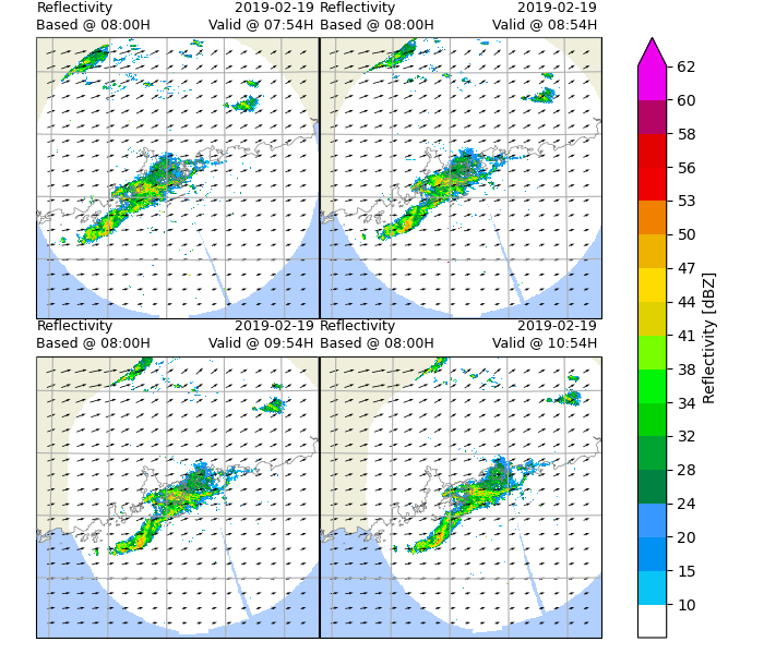
Generating radar reflectivity maps
Define the color scale and format of the plots and plot using xarray.plot().
In this example, only hourly images will be plotted.
# Defining colour scale and format
levels = [
    -32768,
    10, 15, 20, 24, 28, 32,
    34, 38, 41, 44, 47, 50,
    53, 56, 58, 60, 62
]
cmap = ListedColormap([
    '#FFFFFF', '#08C5F5', '#0091F3', '#3898FF', '#008243', '#00A433',
    '#00D100', '#01F508', '#77FF00', '#E0D100', '#FFDC01', '#EEB200',
    '#F08100', '#F00101', '#E20200', '#B40466', '#ED02F0'
])

norm = BoundaryNorm(levels, ncolors=cmap.N, clip=True)

# Defining the crs
crs = area_def_tgt.to_cartopy_crs()

# Generating a timelist for every hour
timelist = [
    (basetime + pd.Timedelta(60*i-6, 'm')) for i in range(4)
]

# Obtaining the slice of the xarray to be plotted
da_plot = reflectivity.sel(time=timelist)

# Defining motion quivers
qx = motion.coords['easting'].values[::5]
qy = motion.coords['northing'].values[::5]
qu = motion.values[0, ::5, ::5]
qv = motion.values[1, ::5, ::5]

# Defining coastlines
map_shape_file = os.path.join(DATA_DIR, "shape/rsmc")
ocean_color = np.array([[[178, 208, 254]]], dtype=np.uint8)
land_color = cfeature.COLORS['land']
coastline = cfeature.ShapelyFeature(
    list(shpreader.Reader(map_shape_file).geometries()),
    ccrs.PlateCarree()
)

# Plotting
p = da_plot.plot(
    col='time', col_wrap=2,
    subplot_kws={'projection': crs},
    cbar_kwargs={
        'extend': 'max',
        'ticks': levels[1:],
        'format': '%.3g'
    },
    cmap=cmap,
    norm=norm
)
for idx, ax in enumerate(p.axes.flat):
    # ocean
    ax.imshow(np.tile(ocean_color, [2, 2, 1]),
              origin='upper',
              transform=ccrs.PlateCarree(),
              extent=[-180, 180, -180, 180],
              zorder=-1)
    # coastline, color
    ax.add_feature(coastline,
                   facecolor=land_color, edgecolor='none', zorder=0)
    # overlay coastline without color
    ax.add_feature(coastline, facecolor='none',
                   edgecolor='gray', linewidth=0.5, zorder=3)
    ax.quiver(qx, qy, qu, qv, pivot='mid', regrid_shape=20)
    ax.gridlines()
    ax.set_title(
        "Reflectivity\n"
        f"Based @ {basetime.strftime('%H:%MH')}",
        loc='left',
        fontsize=9
    )
    ax.set_title(
        ''
    )
    ax.set_title(
        f"{basetime.strftime('%Y-%m-%d')} \n"
        f"Valid @ {timelist[idx].strftime('%H:%MH')} ",
        loc='right',
        fontsize=9
    )
plt.savefig(
    os.path.join(OUTPUT_DIR, "rover-output-map-hk.png"),
    dpi=300
)

radar_image_time = pd.Timestamp.now()
Accumulating hourly rainfall for 3-hour forecast
Hourly accumulated rainfall is calculated every 30 minutes, the first endtime is the basetime i.e. T+0min.
Convert reflectivity in dBZ to rainfalls in 6 mins with to_rainfall_depth().
Changing time coordinates of xarray from start time to endtime.
Accumulate hourly rainfall every 30 minutes using multiple_acc().
# Convert reflectivity to rainrates
rainfalls = to_rainfall_depth(reflectivity, a=58.53, b=1.56)

# Converting the coordinates of xarray from start to endtime
rainfalls.coords['time'] = [
    pd.Timestamp(t) + pd.Timedelta(6, 'm')
    for t in rainfalls.coords['time'].values
]

# Accumulate hourly rainfall every 30 minutes
acc_rf = acc_rainfall_depth(
    rainfalls,
    basetime,
    basetime + pd.Timedelta(hours=3)
)
acc_rf.attrs['long_name'] = 'Rainfall accumulated over the past 60 minutes'

acc_time = pd.Timestamp.now()
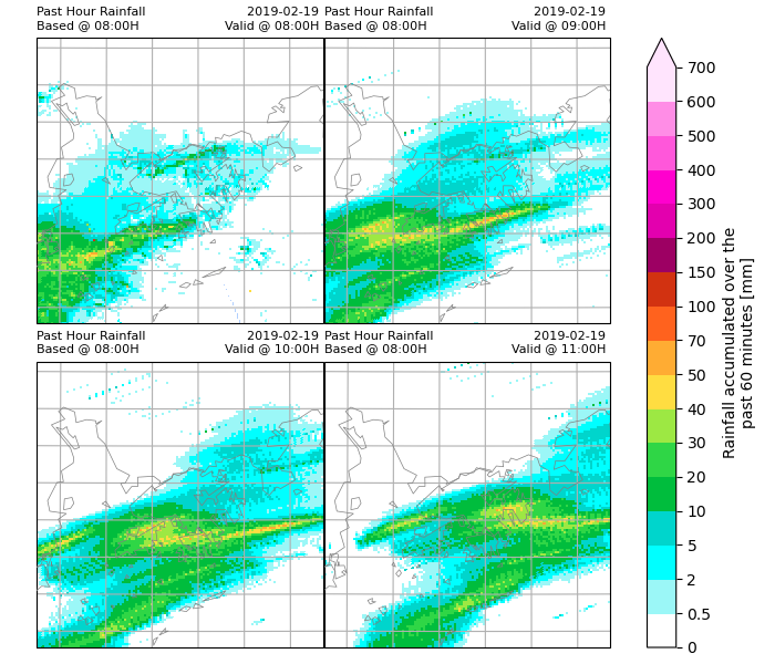
Plotting rainfall maps
Define the colour scheme and format and plot using xarray.plot().
In this example, only hourly images will be plotted.
# Defining the colour scheme
levels = [
    0, 0.5, 2, 5, 10, 20,
    30, 40, 50, 70, 100, 150,
    200, 300, 400, 500, 600, 700
]

cmap = ListedColormap([
    '#ffffff', '#9bf7f7', '#00ffff', '#00d5cc', '#00bd3d', '#2fd646',
    '#9de843', '#ffdd41', '#ffac33', '#ff621e', '#d23211', '#9d0063',
    '#e300ae', '#ff00ce', '#ff57da', '#ff8de6', '#ffe4fd'
])

norm = BoundaryNorm(levels, ncolors=cmap.N, clip=True)

# Defining projection
crs = area_def_tgt.to_cartopy_crs()
# Defining zoom extent
r = 64000
proj_site = acc_rf.proj_site
zoom = (
    proj_site[0]-r, proj_site[0]+r, proj_site[1]-r, proj_site[1]+r
)  # (x0, x1, y0, y1)

# Defining times for plotting
timelist = [basetime + pd.Timedelta(i, 'h') for i in range(4)]

# Obtaining xarray slice to be plotted
da_plot = acc_rf.sel(
    easting=slice(zoom[0], zoom[1]),
    northing=slice(zoom[3], zoom[2]),
    time=timelist
)

# Plotting
p = da_plot.plot(
    col='time', col_wrap=2,
    subplot_kws={'projection': crs},
    cbar_kwargs={
        'extend': 'max',
        'ticks': levels,
        'format': '%.3g'
    },
    cmap=cmap,
    norm=norm
)
for idx, ax in enumerate(p.axes.flat):
    # ocean
    ax.imshow(np.tile(ocean_color, [2, 2, 1]),
              origin='upper',
              transform=ccrs.PlateCarree(),
              extent=[-180, 180, -180, 180],
              zorder=-1)
    # coastline, color
    ax.add_feature(coastline,
                   facecolor=land_color, edgecolor='none', zorder=0)
    # overlay coastline without color
    ax.add_feature(coastline, facecolor='none',
                   edgecolor='gray', linewidth=0.5, zorder=3)
    ax.gridlines()
    ax.set_xlim(zoom[0], zoom[1])
    ax.set_ylim(zoom[2], zoom[3])
    ax.set_title(
        "Past Hour Rainfall\n"
        f"Based @ {basetime.strftime('%H:%MH')}",
        loc='left',
        fontsize=8
    )
    ax.set_title(
        ''
    )
    ax.set_title(
        f"{basetime.strftime('%Y-%m-%d')} \n"
        f"Valid @ {timelist[idx].strftime('%H:%MH')} ",
        loc='right',
        fontsize=8
    )
plt.savefig(
    os.path.join(OUTPUT_DIR, "rainfall_hk.png"),
    dpi=300
)

rf_image_time = pd.Timestamp.now()
Extract the rainfall values at a specified location
In this example, the rainfall values at the location is assumed to be the same as the nearest gridpoint.
Read information regarding the rain gauge stations into a pandas.DataFrame.
Extract the rainfall values at the nearest gridpoint to location for given times (in this example, 30 minute intervals).
Store rainfall values over time in a pandas.DataFrame.
Plot the time series of rainfall at different stations.
# Getting rain gauge station coordinates
df = pd.read_csv(
    os.path.join(DATA_DIR, "hk_raingauge.csv"),
    usecols=[0, 1, 2, 3, 4]
)

# Extract rainfall values at gridpoint closest to the
# location specified for given timesteps and storing it
# in pandas.DataFrame.

rf_time = []
for time in acc_rf.coords['time'].values:
    rf = []
    for index, row in df.iterrows():
        rf.append(acc_rf.sel(
            time=time, northing=row[1],
            easting=row[2],
            method='nearest'
        ).values)
    rf_time.append(rf)

rf_time = np.array(rf_time)

station_rf = pd.DataFrame(
    data=rf_time,
    columns=df.iloc[:, 0],
    index=pd.Index(
        acc_rf.coords['time'].values,
        name='time'
    )
)
print(station_rf)

# Plotting time series graph
ax = station_rf.plot(title="Time Series of Hourly Accumulated Rainfall",
                     grid=True)
ax.set_ylabel("Hourly Accumulated Rainfall (mm)")
plt.savefig(os.path.join(OUTPUT_DIR, "qpf_time_series.png"))

extract_time = pd.Timestamp.now()
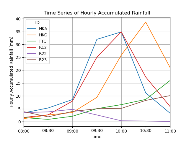
 ID                        HKA        HKO  ...       R22        R23
time                                       ...
2019-02-19 08:00:00   3.147776   1.036804  ...  3.496654   2.518038
2019-02-19 08:30:00   4.966235   2.616592  ...  3.834137   1.678835
2019-02-19 09:00:00   7.267205   2.581846  ...  4.889910   4.395210
2019-02-19 09:30:00  30.130540   7.455962  ...  2.759897   5.611569
2019-02-19 10:00:00  32.616364  26.795704  ...  0.507208   5.566245
2019-02-19 10:30:00   9.996010  40.728087  ...  0.322754   8.934374
2019-02-19 11:00:00   4.845116  21.374541  ...  0.073632  10.662313

[7 rows x 6 columns]
Checking run time of each component
print(f"Start time: {start_time}")
print(f"Initialising time: {initialising_time}")
print(f"Rover time: {rover_time}")
print(f"SLA time: {sla_time}")
print(f"Concatenating time: {concat_time}")
print(f"Plotting radar image time: {radar_image_time}")
print(f"Accumulating rainfall time: {acc_time}")
print(f"Plotting rainfall map time: {rf_image_time}")
print(f"Extracting and plotting time series time: {extract_time}")

print(f"Time to initialise: {initialising_time-start_time}")
print(f"Time to run rover: {rover_time-initialising_time}")
print(f"Time to perform SLA: {sla_time-rover_time}")
print(f"Time to concatenate xarrays: {concat_time - sla_time}")
print(f"Time to plot radar image: {radar_image_time - concat_time}")
print(f"Time to accumulate rainfall: {acc_time - radar_image_time}")
print(f"Time to plot rainfall maps: {rf_image_time-acc_time}")
print(f"Time to extract and plot time series: {extract_time-rf_image_time}")
Start time: 2026-04-20 20:31:58.297716
Initialising time: 2026-04-20 20:32:05.039999
Rover time: 2026-04-20 20:32:05.136737
SLA time: 2026-04-20 20:32:17.667212
Concatenating time: 2026-04-20 20:32:17.724491
Plotting radar image time: 2026-04-20 20:32:48.538799
Accumulating rainfall time: 2026-04-20 20:32:51.261123
Plotting rainfall map time: 2026-04-20 20:32:57.154692
Extracting and plotting time series time: 2026-04-20 20:32:59.401452
Time to initialise: 0 days 00:00:06.742283
Time to run rover: 0 days 00:00:00.096738
Time to perform SLA: 0 days 00:00:12.530475
Time to concatenate xarrays: 0 days 00:00:00.057279
Time to plot radar image: 0 days 00:00:30.814308
Time to accumulate rainfall: 0 days 00:00:02.722324
Time to plot rainfall maps: 0 days 00:00:05.893569
Time to extract and plot time series: 0 days 00:00:02.246760
Total running time of the script: ( 1 minutes 1.197 seconds)