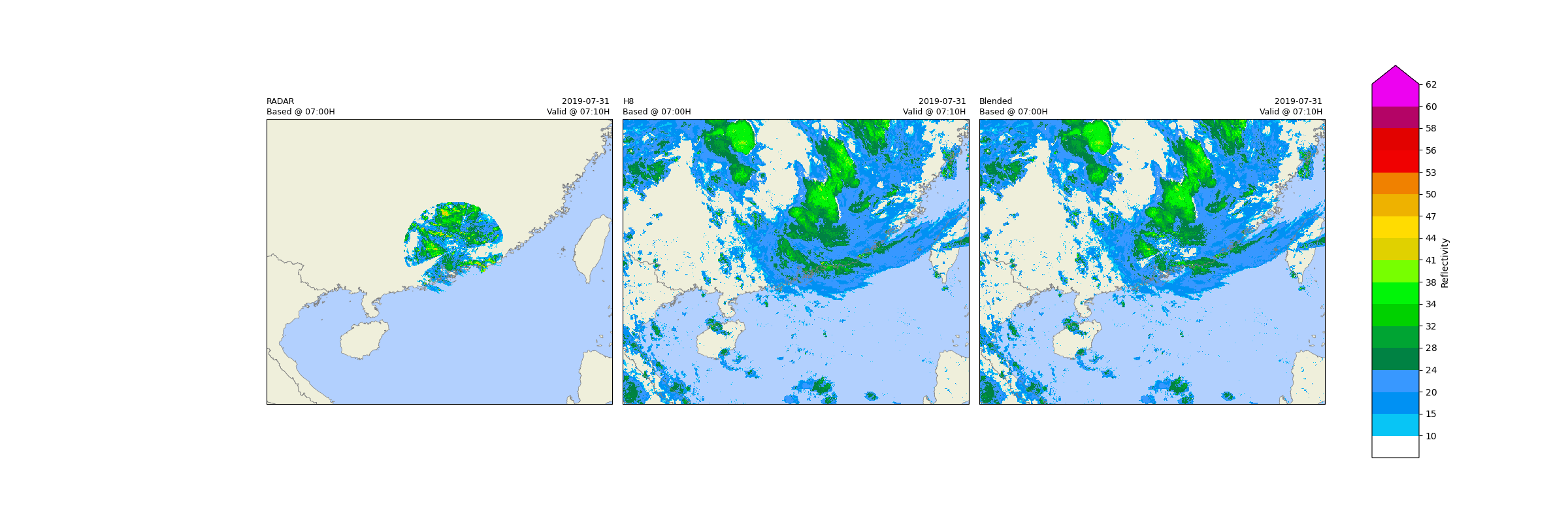
Blending

This example demonstrates how to blend different reflectivity sources into one.

Definitions

Import all required modules and methods:

# Python package to allow system command line functions
import os
# Python package to manage warning message
import warnings
# Python package for time calculations
import pandas as pd
# Python package for numerical calculations
import numpy as np
# Python package for projection
import cartopy.crs as ccrs
# Python package for land/sea features
import cartopy.feature as cfeature
# Python package for reading map shape file
import cartopy.io.shapereader as shpreader
# Python package for creating plots
from matplotlib import pyplot as plt
# Python package for output grid format
from matplotlib.gridspec import GridSpec
# Python package for colorbars
from matplotlib.colors import BoundaryNorm, ListedColormap
from matplotlib.cm import ScalarMappable
# Python package for projection description
from pyresample import get_area_def

# swirlspy regrid function
from swirlspy.core.resample import grid_resample
# swirlspy iris parser function
from swirlspy.rad.iris import read_iris_grid
# swirlspy h8 parser function
from swirlspy.sat.h8 import read_h8_data
# swirlspy blending function
from swirlspy.blending import comp_qpe, Raw
# directory constants
from swirlspy.tests.samples import DATA_DIR
from swirlspy.tests.outputs import OUTPUT_DIR

warnings.filterwarnings("ignore")
plt.switch_backend('agg')

start_time = pd.Timestamp.now()

Initialising

This section demonstrates parsing Himawari-8 data.

Step 1: Define necessary parameter.

# Define base time
base_time = pd.Timestamp("2019-07-31T07:00")

# Define data boundary in WGS84 (latitude)
latitude_from = 30.
latitude_to = 16.
longitude_from = 105.
longitude_to = 122.

area = (
    latitude_from, latitude_to,
    longitude_from, longitude_to
)

# Define grid size, use negative value for descending range
grid_size = (-.025, .025)

# list of source data
sources = []

initialising_time = pd.Timestamp.now()

# Load map shape
map_shape_file = os.path.abspath(os.path.join(DATA_DIR, 'shape/se_asia'))

# coastline and province
map_with_province = cfeature.ShapelyFeature(
    list(shpreader.Reader(map_shape_file).geometries()),
    ccrs.PlateCarree()
)


def plot_base(ax: plt.Axes, extents: list, crs: ccrs.Projection):
    """
    base map function
    """
    ax.set_extent(extents, crs=crs)
    # fake the ocean color
    ax.imshow(
        np.tile(np.array([[[178, 208, 254]]], dtype=np.uint8), [2, 2, 1]),
        origin='upper', transform=ccrs.PlateCarree(),
        extent=[-180, 180, -180, 180], zorder=-1
    )
    # coastline, province and state, color
    ax.add_feature(
        map_with_province, facecolor=cfeature.COLORS['land'],
        edgecolor='none', zorder=0
    )
    # overlay coastline, province and state without color
    ax.add_feature(
        map_with_province, facecolor='none', edgecolor='gray', linewidth=0.5
    )
    ax.set_title('')

Step 2: Read data from radar files into xarray.DataArray using read_iris_grid().

radar = read_iris_grid(os.path.join(DATA_DIR, "iris/RAD190731150000.REF2256"))

radar_time = pd.Timestamp.now()

Step 3: Define the target grid as a pyresample AreaDefinition.

# Defining target grid
area_id = "WGS84"
description = 'World Geodetic System 1984'
proj_id = 'WGS84'
projection = '+proj=longlat +datum=WGS84 +no_defs'
x_size = (longitude_to - longitude_from) / grid_size[1] + 1
y_size = (latitude_to - latitude_from) / grid_size[0] + 1
area_extent = (longitude_from, latitude_from, longitude_to, latitude_to)
radar_area_def = get_area_def(
    area_id, description, proj_id, projection, x_size, y_size, area_extent
)

Step 5: Reproject the radar data from read_iris_grid() from Centered Azimuthal (source) projection to World Geodetic System 1984 projection.

# Extracting the AreaDefinition of the source projection
area_def_src = radar.attrs['area_def']

# Reprojecting
reproj_radar = grid_resample(
    radar, area_def_src, radar_area_def,
    coord_label=['x', 'y']
).sortby(
    ['y'], ascending=False
)

# fix floating point issue
y_coords = np.linspace(
    latitude_from,
    latitude_to,
    reproj_radar.data.shape[1],
    dtype=np.float32
)
x_coords = np.linspace(
    longitude_from,
    longitude_to,
    reproj_radar.data.shape[2],
    dtype=np.float32
)
reproj_radar.coords['y'] = np.array(y_coords)
reproj_radar.coords['x'] = np.array(x_coords)
reproj_radar = reproj_radar.sel(time=reproj_radar.coords['time'].values[0])


radar_site = (
    reproj_radar.attrs['proj_site'][1],
    reproj_radar.attrs['proj_site'][0],
    1.8,  # radius
    0.76  # weight sigma
)

sources.append(Raw(
    reproj_radar,
    [radar_site],  # sites configuration, list of available sites useful for mosaic data
    0.1  # data weight
))

Step 6: Define data directory

# Supply data directory.
# Please make sure H8 data filename is follow the naming pattern -
# HS_H08_{date}_{time}_B{channel:02}_FLDK_R{rsol:02}_S{seg:02}10.DAT
# example:
#   base time = 2019-07-31 07:00 UTC
#   channel = 4
#   resolution = 10
#   segment = 2
#   ========================================
#   filename: HS_H08_20190731_0700_B04_FLDK_R10_S0410.DAT
data_dir = os.path.join(DATA_DIR, "h8")

sat_time = pd.Timestamp.now()

Step 7: Parse data into reflectivity as xarray.DataArray using read_h8_data().

sat = read_h8_data(
    data_dir,
    base_time,
    area,
    grid_size
)
# remove time axis
sat = sat.sel(time=sat.coords['time'].values[0])

# no site data used, treat all points of data with same weight
sources.append(Raw(
    sat,
    weight=0.01  # data weight
))

blend_time = pd.Timestamp.now()

Step 8: Blend all data together.

reflec = comp_qpe(
    grid_size,
    area,
    sources
)


post_time = pd.Timestamp.now()

Step 9: Remove invalid data if needed.

reflec.values[reflec.values < 13.] = reflec.attrs['zero_value']

# update sat data for plotting
sat.values[sat.values < 13.] = sat.attrs['zero_value']

Generating radar reflectivity maps

Define the color scale and format of the plots and plot using xarray.plot().

In this example, only hourly images will be plotted.

# Defining colour scale and format
levels = [
    -32768,
    10, 15, 20, 24, 28, 32,
    34, 38, 41, 44, 47, 50,
    53, 56, 58, 60, 62
]
cmap = ListedColormap([
    '#FFFFFF00', '#08C5F5', '#0091F3', '#3898FF', '#008243', '#00A433',
    '#00D100', '#01F508', '#77FF00', '#E0D100', '#FFDC01', '#EEB200',
    '#F08100', '#F00101', '#E20200', '#B40466', '#ED02F0'
])

norm = BoundaryNorm(levels, ncolors=cmap.N, clip=True)

# colorbar map
mappable = ScalarMappable(cmap=cmap, norm=norm)
mappable.set_array([])

# Defining the crs
crs = ccrs.PlateCarree()
extents = (longitude_from, longitude_to, latitude_from, latitude_to)

# Plotting
fig: plt.Figure = plt.figure(figsize=(24, 8), frameon=False)
gs = GridSpec(
    1, 3, figure=fig, wspace=0.03, hspace=-0.25, top=0.95,
    bottom=0.05, left=0.17, right=0.845
)

# plot radar
ax = fig.add_subplot(gs[0, 0], projection=crs)

plot_base(ax, extents, crs)

im = ax.imshow(reproj_radar.values, cmap=cmap, norm=norm, interpolation='nearest',
               extent=extents)

ax.set_title(
    "RADAR\n"
    f"Based @ {base_time.strftime('%H:%MH')}",
    loc='left',
    fontsize=9
)
ax.set_title(
    ''
)
ax.set_title(
    f"{base_time.strftime('%Y-%m-%d')} \n"
    f"Valid @ {(base_time + pd.Timedelta(minutes=10)).strftime('%H:%MH')} ",
    loc='right',
    fontsize=9
)

# plot H8
ax = fig.add_subplot(gs[0, 1], projection=crs)

plot_base(ax, extents, crs)

im = ax.imshow(sat.values, cmap=cmap, norm=norm, interpolation='nearest',
               extent=extents)

ax.set_title(
    "H8\n"
    f"Based @ {base_time.strftime('%H:%MH')}",
    loc='left',
    fontsize=9
)
ax.set_title(
    ''
)
ax.set_title(
    f"{base_time.strftime('%Y-%m-%d')} \n"
    f"Valid @ {(base_time + pd.Timedelta(minutes=10)).strftime('%H:%MH')} ",
    loc='right',
    fontsize=9
)

# plot blended
ax = fig.add_subplot(gs[0, 2], projection=crs)

plot_base(ax, extents, crs)

im = ax.imshow(reflec.values, cmap=cmap, norm=norm, interpolation='nearest',
               extent=extents)

ax.set_title(
    "Blended\n"
    f"Based @ {base_time.strftime('%H:%MH')}",
    loc='left',
    fontsize=9
)
ax.set_title(
    ''
)
ax.set_title(
    f"{base_time.strftime('%Y-%m-%d')} \n"
    f"Valid @ {(base_time + pd.Timedelta(minutes=10)).strftime('%H:%MH')} ",
    loc='right',
    fontsize=9
)

cbar_ax = fig.add_axes([0.875, 0.125, 0.03, 0.75])
cbar = fig.colorbar(
    mappable, cax=cbar_ax, ticks=levels[1:], extend='max', format='%.3g')
cbar.ax.set_ylabel('Reflectivity', rotation=90)

fig.savefig(
    os.path.join(OUTPUT_DIR, "blending.png"),
    bbox_inches='tight'
)

image_time = pd.Timestamp.now()

Checking run time of each component

print(f"Start time: {start_time}")
print(f"Initialising time: {initialising_time}")
print(f"Read radar time: {radar_time}")
print(f"Parse H8 data time: {sat_time}")
print(f"Blending time: {blend_time}")
print(f"Post blending time: {post_time}")
print(f"Plotting blended image time: {image_time}")

print(f"Time to initialise: {initialising_time - start_time}")
print(f"Time to run read radar: {radar_time - initialising_time}")
print(f"Time to run data parsing: {sat_time - radar_time}")
print(f"Time to run blending: {blend_time - sat_time}")
print(f"Time to perform post process: {post_time - blend_time}")
print(f"Time to plot reflectivity image: {image_time - post_time}")

Start time: 2024-04-18 02:48:05.481088
Initialising time: 2024-04-18 02:48:05.482510
Read radar time: 2024-04-18 02:48:05.808871
Parse H8 data time: 2024-04-18 02:48:06.497071
Blending time: 2024-04-18 02:48:13.646806
Post blending time: 2024-04-18 02:48:13.834524
Plotting blended image time: 2024-04-18 02:48:16.511589
Time to initialise: 0 days 00:00:00.001422
Time to run read radar: 0 days 00:00:00.326361
Time to run data parsing: 0 days 00:00:00.688200
Time to run blending: 0 days 00:00:07.149735
Time to perform post process: 0 days 00:00:00.187718
Time to plot reflectivity image: 0 days 00:00:02.677065