PQPF (Hong Kong)

This example demonstrates how to perform operational PQPF up to three hours from raingauge and radar data, using data from Hong Kong.

Definitions

Import all required modules and methods:

# Python package to allow system command line functions
import os
# Python package to manage warning message
import warnings
# Python package for ordered dictionary
from collections import OrderedDict
# Python package for time calculations
import pandas as pd
# Python package for numerical calculations
import numpy as np
# Python package for xarrays to read and handle netcdf data
import xarray as xr
# Python package for projection description
from pyresample import get_area_def
# Python package for projection
import cartopy.crs as ccrs
# Python package for land/sea features
import cartopy.feature as cfeature
# Python package for reading map shape file
import cartopy.io.shapereader as shpreader
# Python package for creating plots
from matplotlib import pyplot as plt
# Python package for colorbars
from matplotlib.colors import BoundaryNorm, ListedColormap, LinearSegmentedColormap

# Python com-swirls package to calculate motion field (rover) and semi-lagrangian advection
from swirlspy.qpf import rover, sla
# swirlspy data parser function
from swirlspy.rad.iris import read_iris_grid
# swirlspy test data source locat utils function
from swirlspy.qpe.utils import timestamps_ending, locate_file
# swirlspy regrid function
from swirlspy.core.resample import grid_resample
# swirlspy standardize data function
from swirlspy.utils import standardize_attr, FrameType
# swirlspy data convertion function
from swirlspy.utils.conversion import to_rainfall_rate, to_rainfall_depth, acc_rainfall_depth, temporal_interpolate
# directory constants
from swirlspy.tests.samples import DATA_DIR
from swirlspy.tests.outputs import OUTPUT_DIR

warnings.filterwarnings("ignore")
plt.switch_backend('agg')

start_time = pd.Timestamp.now()

Initialising

This section demonstrates extracting radar reflectivity data.

Step 1: Define the basetime.

# Define basetime
basetime = pd.Timestamp('201902190800')

Step 2: Using basetime, generate timestamps of desired radar files timestamps_ending() and locate files using locate_file().

# Obtain radar files
dir = os.path.join(DATA_DIR, 'iris/ppi')
located_files = []
radar_ts = timestamps_ending(
    basetime,
    duration=pd.Timedelta(60, 'm')
)

for timestamp in radar_ts:
    located_files.append(locate_file(dir, timestamp))

Step 3: Read data from radar files into xarray.DataArray using read_iris_grid().

reflectivity_list = []  # stores reflec from read_iris_grid()
for filename in located_files:
    reflec = read_iris_grid(
        filename
    )
    reflectivity_list.append(reflec)

Step 4: Define the target grid as a pyresample AreaDefinition.

# Defining target grid
area_id = "hk1980_250km"
description = ("A 1km resolution rectangular grid "
               "centred at HKO and extending to 250 km "
               "in each direction in HK1980 easting/northing coordinates")
proj_id = 'hk1980'
projection = ('+proj=tmerc +lat_0=22.31213333333334 '
              '+lon_0=114.1785555555556 +k=1 +x_0=836694.05 '
              '+y_0=819069.8 +ellps=intl +towgs84=-162.619,-276.959,'
              '-161.764,0.067753,-2.24365,-1.15883,-1.09425 +units=m '
              '+no_defs')
x_size = 500
y_size = 500
area_extent = (587000, 569000, 1087000, 1069000)
area_def_tgt = get_area_def(
    area_id, description, proj_id, projection, x_size, y_size, area_extent
)

Step 5: Reproject the radar data from read_iris_grid() from Centered Azimuthal (source) projection to HK 1980 (target) projection.

# Extracting the AreaDefinition of the source projection
area_def_src = reflectivity_list[0].attrs['area_def']

# Reprojecting
reproj_reflectivity_list = []
for reflec in reflectivity_list:
    reproj_reflec = grid_resample(
        reflec, area_def_src, area_def_tgt,
        coord_label=['easting', 'northing']
    )
    reproj_reflectivity_list.append(reproj_reflec)

initialising_time = pd.Timestamp.now()

Step 6: Concatenate the reflectivity xarrays in the list along the time dimension.

# Concatenating all the (observed) reflectivity
# xarray.DataArrays in reproj_reflectivity_list
reflectivityObs = xr.concat(reproj_reflectivity_list, dim='time')

Running ROVER and Semi-Lagrangian Advection

This section demonstrates how to run ROVER and Semi-Lagrangian Advection for multiple members.

First, write a function to run these steps:

1. Selecting the two relevant xarrays to be used as the ROVER input.

2. Generate motion field using ROVER, with the selected xarray as the input.

3. Perform Semi-Lagrangian Advection using the motion fields from ROVER.

Writing the function makes it easier to implement multiprocessing if required.

def ensemble_rover_sla(
    reflectivityObs,
    basetime,
    interval,
    duration,
    member,
    start_level,
    max_level,
    rho, alpha, sigma,
    track_interval
):
    """
    A function to run ROVER and SLA.

    Parameters
    -------------
    reflectivityObs: xarray.DataArray
        The xarray containing observed reflectivity.
    basetime: pandas.Timestamp
        The basetime of the forecast.
        Equivalent to the end time of the latest radar scan.
    interval: pandas.Timedelta
        The interval between the radar scans.
    duration: pandas.Timedelta
        The duration of the forecast.
    member: str
        The name of the member.
    start_level, max_level, rho, alpha, sigma, track_interval: floats
        Parameters of the members.

    Returns
    ------------
    reflectivityFcst: xarray.DataArray
        Contains foreacsted reflectivity.
    """

    # Generate timestamps of relevant radar scans
    latestRadarScanTime = basetime - interval

    roverTimestrings = timestamps_ending(
        latestRadarScanTime, duration=track_interval,
        interval=track_interval,
        format='%Y%m%d%H%M',
        exclude_end=False
    )

    roverTimestamps = [pd.Timestamp(t) for t in roverTimestrings]

    qpf_xarray = reflectivityObs.sel(time=roverTimestamps)
    standardize_attr(qpf_xarray, frame_type=FrameType.dBZ, zero_value=9999.0)

    # Generate motion field using ROVER
    motion = rover(
        qpf_xarray,
        start_level=start_level,
        max_level=max_level,
        rho=rho,
        sigma=sigma,
        alpha=alpha
    )

    # Perform SLA
    steps = int(duration / interval)
    reflectivityFcst = sla(qpf_xarray, motion, steps)

    reflectivityFcst = reflectivityFcst.expand_dims(
        dim=OrderedDict({'member': [member]})
    ).copy()

    return reflectivityFcst

Then, run the different members by calling the function above. In this example. only four members are run.

# Define the member parameters
# Ensure that values at the same position across
# the tuples correspond to the same member
startLevelTuple = (1, 2, 1, 1)
maxLevelTuple = (7, 7, 7, 7)
sigmaTuple = (2.5, 2.5, 1.5, 1.5)
rhoTuple = (9., 9., 9., 9.)
alphaTuple = (2000., 2000., 2000., 2000.)
memberTuple = ('Mem-1', 'Mem-2', 'Mem-3', 'Mem-4')
trackIntervalList = [pd.Timedelta(i, 'm') for i in [6, 12, 6, 12]]

processes = 4

reflectivityFcstList = []
for i in range(processes):
    args = (
        reflectivityObs,
        basetime,
        pd.Timedelta(6, 'm'),
        pd.Timedelta(3, 'h'),
        memberTuple[i],
        startLevelTuple[i],
        maxLevelTuple[i],
        rhoTuple[i],
        alphaTuple[i],
        sigmaTuple[i],
        trackIntervalList[i]
    )
    reflectivityFcst = ensemble_rover_sla(*args)
    reflectivityFcstList.append(reflectivityFcst)

rover_sla_time = pd.Timestamp.now()

RUNNING 'rover' FOR EXTRAPOLATION.....
RUNNING 'rover' FOR EXTRAPOLATION.....
RUNNING 'rover' FOR EXTRAPOLATION.....
RUNNING 'rover' FOR EXTRAPOLATION.....

Concatenating observed and forecasted reflectivities

From the results from all members:

1. Change the timestamps of observed reflectivity and forecasted reflectivity of all members from start time to end time.

2. Add forecasted reflectivity to reproj_reflectivity_list.

3. Concatenate observed and forecasted reflectivity xarray.DataArrays along the time dimension.

# List to store combined reflectivity arrays of each member
reflectivityConcatList = []

# Changing the time coordinates from start time to end time
reflectivityObs.coords['time'] = [
    pd.Timestamp(t) + pd.Timedelta(6, 'm')
    for t in reflectivityObs.time.values
]

for reflectivityFcst in reflectivityFcstList:
    # Identify the member
    member = reflectivityFcst.member.values[0]
    # Add member dimension to observed reflectivity
    reflectivityObsExpanded = reflectivityObs.expand_dims(
        dim=OrderedDict({'member': [member]})
    ).copy()

    # Checking for the track interval of the forecasted
    # array
    timeIntervalsSet = set(np.diff(reflectivityFcst.time.values))
    if pd.Timedelta(12, 'm').to_timedelta64() in timeIntervalsSet:
        reflectivityFcst.coords['time'] = [
            pd.Timestamp(t) + pd.Timedelta(12, 'm')
            for t in reflectivityFcst.time.values
        ]
    else:
        reflectivityFcst.coords['time'] = [
            pd.Timestamp(t) + pd.Timedelta(6, 'm')
            for t in reflectivityFcst.time.values
        ]

    # Combining
    reflectivityList = [
        reflectivityObsExpanded,
        reflectivityFcst.isel(time=slice(1, None))
    ]
    reflectivity = xr.concat(reflectivityList, dim='time')
    standardize_attr(reflectivity, frame_type=FrameType.dBZ,
                     zero_value=reflectivityFcst.attrs['zero_value'])
    reflectivityConcatList.append(reflectivity)

concat_time = pd.Timestamp.now()

Accumulating hourly rainfall for 3-hour forecast

Hourly accumulated rainfall is calculated every 30 minutes, the first endtime is the basetime i.e. T+0min.

1. Convert reflectivity in dBZ to rainrates in mm/h with dbz2rr().

2. For rainrates every 12 minutes, interpolate rainfall temporally to once every 6 minutes to ensure that rainrates are equally spaced along the time axis.

3. Convert rainrates to rainfalls with rr2rf().

4. Compute hourly accumulated rainfall every 30 minutes.

5. Concatenate accumulated rainfall of different members along the member dimension.

accList = []
for reflectivity in reflectivityConcatList:
    # Converting reflectivity to rainrates
    rainrates = to_rainfall_rate(
        reflectivity, logarithmic=False, a=58.53, b=1.56)

    # Interpolate rainfall to every 12 minutes if
    # the member has a track interval of 12 minutes
    if pd.Timedelta(12, 'm').to_timedelta64() in timeIntervalsSet:
        rainrates = temporal_interpolate(rainrates,
                                         basetime - pd.Timedelta(1, 'h'),
                                         basetime + pd.Timedelta(3, 'h'),
                                         pd.Timedelta(6, 'm'),
                                         'linear')
    # Convert rainrates to rainfalls every 6 minutes
    rainfalls = to_rainfall_depth(rainrates)

    # Accumulate rainfalls every 30 minutes
    accr = acc_rainfall_depth(rainfalls,
                              basetime,
                              basetime + pd.Timedelta(3, 'h'),
                              pd.Timedelta(30, 'm'),
                              pd.Timedelta(1, 'h'))
    accList.append(accr)

# Concatenating along the mmeber dimension
acc_rf = xr.concat(accList, dim='member')

acc_time = pd.Timestamp.now()

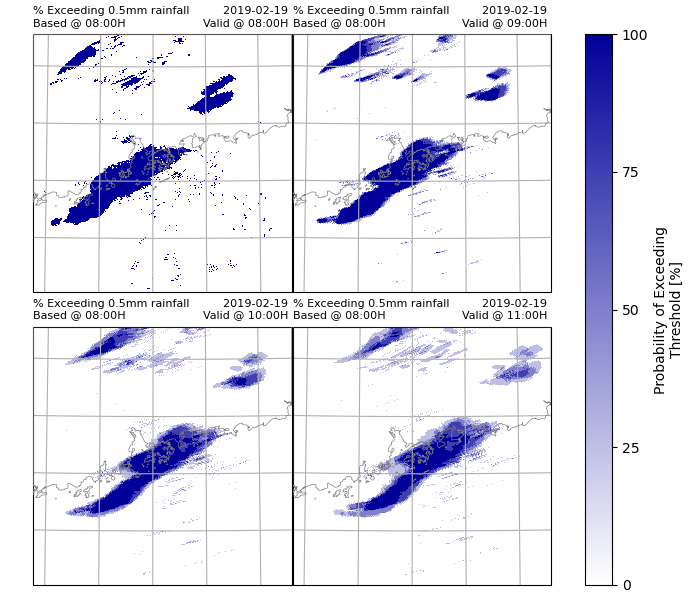
Calculating Probability Exceeding Threshold

In this example, thresholds are 0.5mm, 5mm, 10mm, 30mm, 50mm and 70 mm.

Probabilities are 0%, 25%, 50%, 75% and 100%, as there are four members.

Steps:

1. Define threshold.

2. Use a loop to calculate the probability of exceeding threshold for each gridcell and store results in list.

3. Concatenate the contents of the list. Result is an xarray with dimensions (threshold, time, y, x).

4. Plot the results using xarray.plot(). In this example, only the probability exceeding 0.5mm rainfall every hour will be plotted.

# Define threshold
threshold = [0.5, 5., 10., 30., 50., 70.]

# Define list to store probabilities of exceeding rainfall thresholds
# List corresponds to threshold
prob_list = []

# Calculate probability
for th in threshold:
    bool_forecast = acc_rf >= th
    count = bool_forecast.sum(dim='member')
    prob = count/len(bool_forecast.coords['member'].values) * 100
    prob_list.append(prob)

# Generate coordinate xarray for threshold
th_xarray = xr.IndexVariable('threshold', threshold)

# concatenate
prob_rainfall = xr.concat(prob_list, dim=th_xarray)

prob_rainfall.attrs['long_name'] = "Probability of Exceeding Threshold"
prob_rainfall.attrs['units'] = "%"

# Plot the results

# Extracting the crs
crs = area_def_tgt.to_cartopy_crs()

# Defining cmap
cmap = LinearSegmentedColormap.from_list(
    'custom blue', ['#FFFFFF', '#000099']
)

# Obtaining xarray slices to be plotted
threshold_list = [0.5]
timelist = [basetime + pd.Timedelta(hours=i) for i in range(4)]
da_plot = prob_rainfall.sel(threshold=threshold_list, time=timelist)

# Defining coastlines
map_shape_file = os.path.join(DATA_DIR, "shape/rsmc")
ocean_color = np.array([[[178, 208, 254]]], dtype=np.uint8)
land_color = cfeature.COLORS['land']
coastline = cfeature.ShapelyFeature(
    list(shpreader.Reader(map_shape_file).geometries()),
    ccrs.PlateCarree()
)

for th in threshold_list:
    # Plotting
    p = da_plot.sel(threshold=th).plot(
        col='time', col_wrap=2,
        subplot_kws={'projection': crs},
        cbar_kwargs={'ticks': [0, 25, 50, 75, 100],
                     'format': '%.3g'},
        cmap=cmap
    )

    for idx, ax in enumerate(p.axes.flat):
        # ocean
        ax.imshow(np.tile(ocean_color, [2, 2, 1]),
                  origin='upper',
                  transform=ccrs.PlateCarree(),
                  extent=[-180, 180, -180, 180],
                  zorder=-1)
        # coastline, color
        ax.add_feature(coastline,
                       facecolor=land_color, edgecolor='none', zorder=0)
        # overlay coastline without color
        ax.add_feature(coastline, facecolor='none',
                       edgecolor='gray', linewidth=0.5, zorder=3)
        ax.gridlines()  # gridlines
        ax.set_title(
            f"% Exceeding {th}mm rainfall\n"
            f"Based @ {basetime.strftime('%H:%MH')}",
            loc='left',
            fontsize=8
        )
        ax.set_title(
            ''
        )
        ax.set_title(
            f"{basetime.strftime('%Y-%m-%d')} \n"
            f"Valid @ {timelist[idx].strftime('%H:%MH')} ",
            loc='right',
            fontsize=8
        )
    plt.savefig(
        os.path.join(OUTPUT_DIR, f"p_{th}.png"),
        dpi=300
    )

prob_time = pd.Timestamp.now()

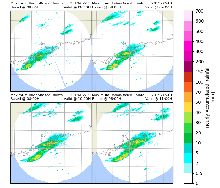
Rainfall percentiles

1. Using xarray.DataArray.mean(), calculate the mean rainfall of all gridpoints.

2. Using xarray.DataArray.min(), find the minimum rainfall of all gridpoints.

3. Using xarray.DataArray.max(), find the maximum rainfall of all gridpoints.

4. Using xarray.DataArray.quantile() find the 25th, 50th and 75th percentile rainfall of all gridpoints.

5. Concatenate rainfall along percentile dimension.

6. Plot results using xarray.plot(). In this example only the maximum percentile rainfall every hour will be plotted.

# mean
mean_rainfall = acc_rf.mean(dim='member', keep_attrs=True)
# max
max_rainfall = acc_rf.max(dim='member', keep_attrs=True)
# min
min_rainfall = acc_rf.min(dim='member', keep_attrs=True)
# quartiles
q_rainfall = acc_rf.quantile(
    [.25, .5, .75], dim='member',
    interpolation='nearest', keep_attrs=True)

# generate index
percentile = xr.IndexVariable(
    'percentile',
    ['Minimum',
     '25th Percentile',
     '50th Percentile',
     'Mean',
     '75th Percentile',
     'Maximum']
)

# concatenating

p_rainfall = xr.concat(
    [min_rainfall,
     q_rainfall.sel(quantile=.25).squeeze().drop('quantile'),
     q_rainfall.sel(quantile=.50).squeeze().drop('quantile'),
     mean_rainfall,
     q_rainfall.sel(quantile=.75).squeeze().drop('quantile'),
     max_rainfall],
    dim=percentile
)

p_rainfall.attrs['long_name'] = "Hourly Accumulated Rainfall"
p_rainfall.attrs['units'] = "mm"

# Defining levels

# Defining the colour scheme
levels = [
    0, 0.5, 2, 5, 10, 20,
    30, 40, 50, 70, 100, 150,
    200, 300, 400, 500, 600, 700
]

cmap = ListedColormap([
    '#ffffff', '#9bf7f7', '#00ffff', '#00d5cc', '#00bd3d', '#2fd646',
    '#9de843', '#ffdd41', '#ffac33', '#ff621e', '#d23211', '#9d0063',
    '#e300ae', '#ff00ce', '#ff57da', '#ff8de6', '#ffe4fd'
])

norm = BoundaryNorm(levels, ncolors=cmap.N, clip=True)

# Obtaining xarray slices to be plotted
plot_positions = ['Maximum']
timelist = [basetime + pd.Timedelta(hours=i) for i in range(4)]
da_plot = p_rainfall.sel(percentile=plot_positions, time=timelist)

for pos in plot_positions:
    # Plotting
    p = da_plot.sel(percentile=pos).plot(
        col='time', col_wrap=2,
        subplot_kws={'projection': crs},
        cbar_kwargs={'ticks': levels,
                     'format': '%.3g'},
        cmap=cmap,
        norm=norm
    )

    for idx, ax in enumerate(p.axes.flat):
        # ocean
        ax.imshow(np.tile(ocean_color, [2, 2, 1]),
                  origin='upper',
                  transform=ccrs.PlateCarree(),
                  extent=[-180, 180, -180, 180],
                  zorder=-1)
        # coastline, color
        ax.add_feature(coastline,
                       facecolor=land_color, edgecolor='none', zorder=0)
        # overlay coastline without color
        ax.add_feature(coastline, facecolor='none',
                       edgecolor='gray', linewidth=0.5, zorder=3)
        ax.gridlines()
        ax.set_title(
            f"{pos} Radar-Based Rainfall\n"
            f"Based @ {basetime.strftime('%H:%MH')}",
            loc='left',
            fontsize=8
        )
        ax.set_title(
            ''
        )
        ax.set_title(
            f"{basetime.strftime('%Y-%m-%d')} \n"
            f"Valid @ {timelist[idx].strftime('%H:%MH')} ",
            loc='right',
            fontsize=8
        )
        position = pos.split(" ")[0]
    plt.savefig(
        os.path.join(OUTPUT_DIR, f"rainfall_{position}.png"),
        dpi=300
    )
ptime = pd.Timestamp.now()

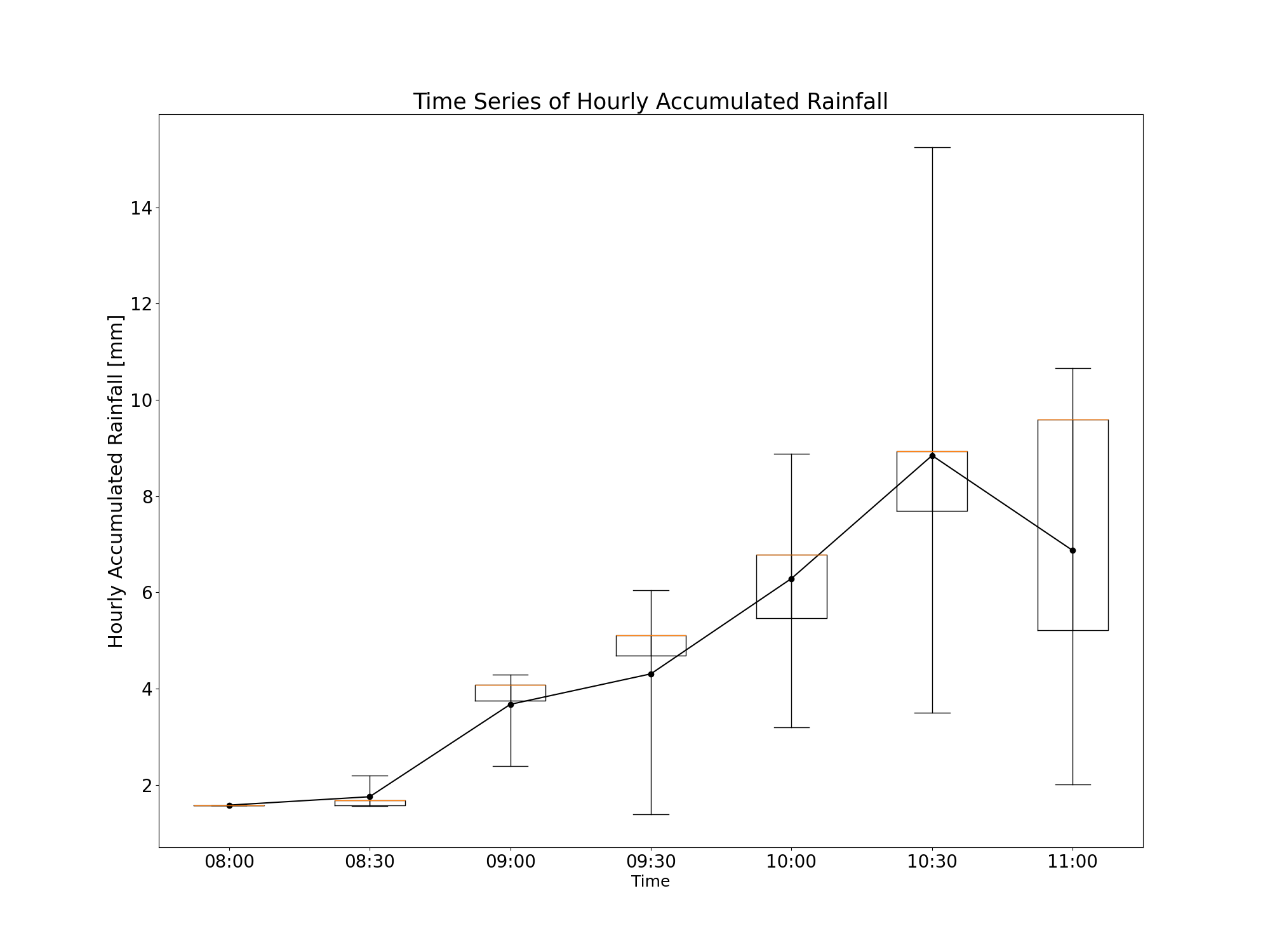
Extract the rainfall values at a specified location

In this example, the rainfall values at the location is assumed to be the same as the nearest gridpoint.

1. Read information regarding the radar stations into a pandas.DataFrame.

2. Extract the rainfall values at the nearest gridpoint to location for given timesteps (in this example, 30 minute intervals).

3. Store rainfall values over time in an xarray.DataArray.

4. Plot the time series of rainfall with boxplots at desired station. In this case, the 15th percentile member is plotted.

# Getting radar station coordinates
df = pd.read_csv(
    os.path.join(DATA_DIR, "hk_raingauge.csv"),
    usecols=[0, 1, 2, 3, 4]
)

# Extract rainfall values at gridpoint closest to the
# location specified for given timesteps and storing it
# in xarray.DataArray.
station_rf_list = []
station_name = []
for index, row in df.iterrows():
    station_rf_list.append(p_rainfall.sel(
        northing=row[1], easting=row[2],
        method='nearest'
    ).drop('northing').drop('easting'))
    station_name.append(row[0])

station_name_index = xr.IndexVariable(
    'ID', station_name
)
station_rf = xr.concat(
    station_rf_list,
    dim=station_name_index
)

# Extracting the 15th ranked station
xr_15_percentile = station_rf.quantile(
    .15, dim='ID', interpolation='nearest').drop('quantile')

# Plotting
_, tax = plt.subplots(figsize=(20, 15))
plt.plot(
    np.arange(1, len(xr_15_percentile.coords['time'].values) + 1),
    xr_15_percentile.loc['Mean'].values,
    'ko-'
)  # plot line

# Storing percentiles as dictionary to call ax.bxp for boxplot
stats_list = []
for i in range(len(xr_15_percentile.coords['time'].values)):
    stats = {
        'med': xr_15_percentile.loc['50th Percentile'].values[i],
        'q1': xr_15_percentile.loc['25th Percentile'].values[i],
        'q3': xr_15_percentile.loc['75th Percentile'].values[i],
        'whislo': xr_15_percentile.loc['Maximum'].values[i],
        'whishi': xr_15_percentile.loc['Minimum'].values[i]
    }
    stats_list.append(stats)

# Plot boxplot
tax.bxp(
    stats_list, showfliers=False
)

# Labels
xcoords = xr_15_percentile.coords['time'].values
xticklabels = [pd.to_datetime(str(t)).strftime("%H:%M") for t in xcoords]
tax.set_xticklabels(xticklabels)
tax.xaxis.set_tick_params(labelsize=20)
tax.yaxis.set_tick_params(labelsize=20)
plt.title('Time Series of Hourly Accumulated Rainfall', fontsize=25)
plt.ylabel("Hourly Accumulated Rainfall [mm]", fontsize=22)
plt.xlabel("Time", fontsize=18)
plt.savefig(
    os.path.join(OUTPUT_DIR, "pqpf_time_series.png")
)

extract_time = pd.Timestamp.now()

Checking run time of each component

print(f"Start time: {start_time}")
print(f"Initialising time: {initialising_time}")
print(f"Rover and SLA time: {rover_sla_time}")
print(f"Concatenating time: {concat_time}")
print(f"Accumulating rainfall time: {acc_time}")
print("Calculate and plot probability exceeding threshold: "
      f"{prob_time}")
print(f"Plotting rainfall maps: {ptime}")
print(f"Extracting and plotting time series time: {extract_time}")

print(f"Time to initialise: {initialising_time-start_time}")
print(f"Time to run rover and SLA: {rover_sla_time-initialising_time}")
print(f"Time to concatenate xarrays: {concat_time - rover_sla_time}")
print(f"Time to accumulate rainfall: {acc_time - concat_time}")
print("Time to calculate and plot probability exceeding threshold: "
      f"{prob_time-acc_time}")
print(f"Time to plot rainfall maps: {ptime-prob_time}")
print(f"Time to extract station data and plot time series: "
      f"{extract_time-ptime}")

Start time: 2024-04-22 04:21:59.879182
Initialising time: 2024-04-22 04:22:06.329826
Rover and SLA time: 2024-04-22 04:23:24.488999
Concatenating time: 2024-04-22 04:23:24.681257
Accumulating rainfall time: 2024-04-22 04:23:28.926826
Calculate and plot probability exceeding threshold: 2024-04-22 04:23:38.139917
Plotting rainfall maps: 2024-04-22 04:25:07.993525
Extracting and plotting time series time: 2024-04-22 04:25:09.830708
Time to initialise: 0 days 00:00:06.450644
Time to run rover and SLA: 0 days 00:01:18.159173
Time to concatenate xarrays: 0 days 00:00:00.192258
Time to accumulate rainfall: 0 days 00:00:04.245569
Time to calculate and plot probability exceeding threshold: 0 days 00:00:09.213091
Time to plot rainfall maps: 0 days 00:01:29.853608
Time to extract station data and plot time series: 0 days 00:00:01.837183