QPF (Thailand)

This example demonstrates how to perform operational deterministic QPF up to three hours from hourly composite rainfall data, using data from Thailand.

Definitions

Import all required modules and methods:

# Python package to allow system command line functions
import os
# Python package to manage warning message
import warnings
# Python package for time calculations
import pandas as pd
# Python package for numerical calculations
import numpy as np
# Python package for xarrays to read and handle netcdf data
import xarray as xr
# Python package for projection
import cartopy.crs as ccrs
# Python package for land/sea features
import cartopy.feature as cfeature
# Python package for reading map shape file
import cartopy.io.shapereader as shpreader
# Python package for creating plots
from matplotlib import pyplot as plt
# Python package for projection conversion
from utm.conversion import from_latlon
# Python package for colorbars
from matplotlib.colors import BoundaryNorm, ListedColormap
# Python package for area definition
from pyresample import get_area_def

# Python com-swirls package to calculate motion field (rover) and semi-lagrangian advection
from swirlspy.qpf import rover, sla
# swirlspy Thailand netcdf file parser function
from swirlspy.rad import read_netcdf_th_refl
# swirlspy regrid function
from swirlspy.core.resample import grid_resample
# swirlspy standardize data function
from swirlspy.utils import standardize_attr, FrameType
# swirlspy data convertion function
from swirlspy.utils.conversion import to_rainfall_depth, acc_rainfall_depth
# directory constants
from swirlspy.tests.samples import DATA_DIR
from swirlspy.tests.outputs import OUTPUT_DIR

warnings.filterwarnings("ignore")
plt.switch_backend('agg')

start_time = pd.Timestamp.now()

Initialising

This section demonstrates extracting radar reflectivity data.

Step 1: Define a basetime.

# Supply basetime
baseT = "202010161000"
basetime = pd.Timestamp(baseT)

Step 2: Using basetime, generate timestamps of desired radar files.

# Obtain radar files
located_files = []
interval = pd.Timedelta(15, 'm')
duration = pd.Timedelta(60, 'm')

while duration >= pd.Timedelta(0):
    located_files.append(
        os.path.abspath(os.path.join(
            DATA_DIR,
            'netcdf_tmd',
            (basetime - duration).strftime('RADAR_Thailand2_%Y%m%dT%H%M%S000Z.nc')
        )
        ))
    duration -= interval

Step 3: Read data from radar files into xarray.DataArray using read_netcdf_th_refl().

# defining the a and b value of the Z-R relationship
ZRa = 300
ZRb = 1.4


reflect_list = []  # stores reflectivity from read_netcdf_th-refl()
for filename in located_files:
    reflec = read_netcdf_th_refl(
        filename, ZRa, ZRb
    )
    reflect_list.append(reflec)

Step 4 : Define the target grid

Defining target grid

area_id = "Thai1975"
description = ("Covering whole territory of Thailand")
proj_id = 'Thai'
projection = "+proj=utm +zone=47 +a=6377276.345 +b=6356075.41314024 +towgs84=210,814,289,0,0,0,0 +units=m +no_defs "
x_size = len(reflect_list[0][0][0])
y_size = len(reflect_list[0][0][:])

lon = reflect_list[0][0][0].coords['lon']
lat = reflect_list[0][0].coords['lat']

# Using utm to calculate the coordinate system
ll = from_latlon(float(lat[-1]), float(lon[0]), 47)
ur = from_latlon(float(lat[0]), float(lon[-1]), 47)

area_extent = (ll[0], ll[1], ur[0], ur[1])

area_def_tgt = get_area_def(
    area_id, description, proj_id, projection, x_size, y_size, area_extent
)

Step 5: Reproject the radar data from read_netcdf_th_refl() (source) projection to Thai (target) projection.

# Extracting the AreaDefinition of the source projection

area_def_src = reflect_list[0].attrs['area_def']

reproj_reflect_list = []
for reflect in reflect_list:
    reproj_reflect = grid_resample(
        reflect, area_def_src, area_def_tgt,
        coord_label=['easting', 'northing']
    )
    reproj_reflect_list.append(reproj_reflect)

Step 6: Assigning reflectivity xarrays at the last two timestamps to variables for use during ROVER QPF.

initialising_time = pd.Timestamp.now()

Running ROVER and Semi-Lagrangian Advection

1. Concatenate two reflectivity xarrays along time dimension.

2. Run ROVER, with the concatenated xarray as the input.

3. Perform Semi-Lagrangian Advection using the motion fields from rover.

# Combining the two reflectivity DataArrays
# the order of the coordinate keys is now ['y', 'x', 'time']
# as opposed to ['time', 'x', 'y']

reflect_concat = xr.concat(reproj_reflect_list, dim='time')
standardize_attr(reflect_concat, frame_type=FrameType.dBZ, zero_value=9999.)


# Rover
motion = rover(reflect_concat)

rover_time = pd.Timestamp.now()


# Semi Lagrangian Advection
reflectivity = sla(reflect_concat, motion, 12)

sla_time = pd.Timestamp.now()

RUNNING 'rover' FOR EXTRAPOLATION.....

Concatenating observed and forecasted reflectivities

1. Add forecasted reflectivity to reproj_reflectivity_list.

2. Concatenate observed and forecasted reflectivity xarray.DataArrays along the time dimension.

reflectivity = xr.concat([reflect_concat[:-1, ...], reflectivity], dim='time')
reflectivity.attrs['long_name'] = '2 km radar composite reflectivity'
standardize_attr(reflectivity)

concat_time = pd.Timestamp.now()

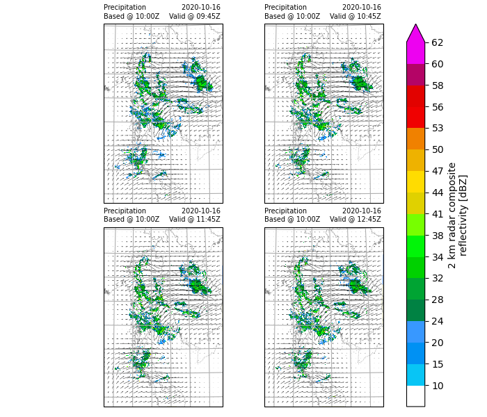
Generating radar reflectivity maps

Define the color scale and format of the plots and plot using xarray.plot().

In this example, only hourly images will be plotted.

# Defining colour scale and format
levels = [
    -32768,
    10, 15, 20, 24, 28, 32,
    34, 38, 41, 44, 47, 50,
    53, 56, 58, 60, 62
]
cmap = ListedColormap([
    '#FFFFFF', '#08C5F5', '#0091F3', '#3898FF', '#008243', '#00A433',
    '#00D100', '#01F508', '#77FF00', '#E0D100', '#FFDC01', '#EEB200',
    '#F08100', '#F00101', '#E20200', '#B40466', '#ED02F0'
])


norm = BoundaryNorm(levels, ncolors=cmap.N, clip=True)

# Defining the crs
crs = area_def_tgt.to_cartopy_crs()

# Defining coastlines
map_shape_file = os.path.join(DATA_DIR, "shape/rsmc")
ocean_color = np.array([[[178, 208, 254]]], dtype=np.uint8)
land_color = cfeature.COLORS['land']
coastline = cfeature.ShapelyFeature(
    list(shpreader.Reader(map_shape_file).geometries()),
    ccrs.PlateCarree()
)

# Generating a timelist for every hour
timelist = [
    (basetime + pd.Timedelta(minutes=60*i-15)) for i in range(4)
]


# Obtaining the slice of the xarray to be plotted
da_plot = reflectivity.sel(time=timelist)


# Defining motion quivers
qx = motion.coords['easting'].values[::50]
qy = motion.coords['northing'].values[::50]
qu = motion.values[0, ::50, ::50]
qv = motion.values[1, ::50, ::50]

# Plotting
p = da_plot.plot(
    col='time', col_wrap=2,
    subplot_kws={'projection': crs},
    cbar_kwargs={
        'extend': 'max',
        'ticks': levels[1:],
        'format': '%.3g'
    },
    cmap=cmap,
    norm=norm
)


for idx, ax in enumerate(p.axes.flat):
    # ocean
    ax.imshow(np.tile(ocean_color, [2, 2, 1]),
              origin='upper',
              transform=ccrs.PlateCarree(),
              extent=[-180, 180, -180, 180],
              zorder=-1)
    # coastline, color
    ax.add_feature(coastline,
                   facecolor=land_color, edgecolor='none', zorder=0)
    # overlay coastline without color
    ax.add_feature(coastline, facecolor='none',
                   edgecolor='gray', linestyle=':', linewidth=0.5)
    # precipitation
    ax.quiver(qx, qy, qu, qv, pivot='mid', scale=20, scale_units='inches')
    ax.gridlines()
    ax.set_title(
        "Precipitation\n"
        f"Based @ {basetime.strftime('%H:%MZ')}",
        loc='left',
        fontsize=7
    )
    ax.set_title(
        ''
    )
    ax.set_title(
        f"{basetime.strftime('%Y-%m-%d')} \n"
        f"Valid @ {timelist[idx].strftime('%H:%MZ')} ",
        loc='right',
        fontsize=7
    )


plt.savefig(
    os.path.join(OUTPUT_DIR, f"rover-output-map-mn{baseT}.png"),
    dpi=300
)

radar_image_time = pd.Timestamp.now()

Accumulating hourly rainfall for 3-hour forecast

Hourly accumulated rainfall is calculated every 30 minutes, the first endtime is the basetime i.e. T+0min.

1. Convert reflectivity in dBZ to rainfalls in 6 mins with to_rainfall_depth().

2. Changing time coordinates of xarray from start time to endtime.

3. Accumulate hourly rainfall every 30 minutes using multiple_acc().

# Convert reflectivity to rainrates
rainfalls = to_rainfall_depth(reflectivity, a=ZRa, b=ZRb)

# Converting the coordinates of xarray from start to endtime
rainfalls.coords['time'] = [
    pd.Timestamp(t) + pd.Timedelta(15, 'm')
    for t in rainfalls.coords['time'].values
]


intervalstep = 30
result_step_size = pd.Timedelta(minutes=intervalstep)


# Accumulate hourly rainfall every 30 minutes
acc_rf = acc_rainfall_depth(
    rainfalls,
    basetime,
    basetime + pd.Timedelta(hours=3),
    result_step_size=result_step_size
)
acc_rf.attrs['long_name'] = 'Rainfall accumulated over the past 60 minutes'


acc_time = pd.Timestamp.now()


# Defining times for plotting
timelist = [basetime + pd.Timedelta(i, 'h') for i in range(4)]

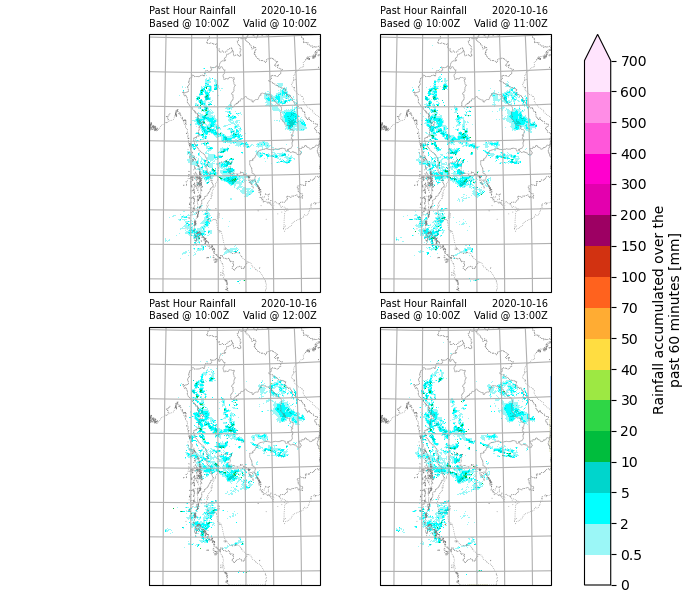
Plotting rainfall maps

Define the colour scheme and format and plot using xarray.plot().

In this example, only hourly images will be plotted.

# Defining the colour scheme
levels2 = [
    0.,  0.5,   2.,   5.,  10.,  20.,
    30.,  40.,  50.,  70., 100., 150.,
    200., 300., 400., 500., 600., 700.
]

cmap2 = ListedColormap([
    '#ffffff', '#9bf7f7', '#00ffff', '#00d5cc', '#00bd3d', '#2fd646',
    '#9de843', '#ffdd41', '#ffac33', '#ff621e', '#d23211', '#9d0063',
    '#e300ae', '#ff00ce', '#ff57da', '#ff8de6', '#ffe4fd'
])

norm2 = BoundaryNorm(levels2, ncolors=cmap2.N, clip=True)

# Defining times for plotting
timelist = [basetime + pd.Timedelta(i, 'h') for i in range(4)]

# Obtaining xarray slice to be plotted
da_plot = acc_rf.sel(
    time=timelist
)

# Plotting
p = da_plot.plot(
    col='time', col_wrap=2,
    subplot_kws={'projection': crs},
    cbar_kwargs={
        'extend': 'max',
        'ticks': levels2,
        'format': '%.3g'
    },
    cmap=cmap2,
    norm=norm2
)
for idx, ax in enumerate(p.axes.flat):
    # ocean
    ax.imshow(np.tile(ocean_color, [2, 2, 1]),
              origin='upper',
              transform=ccrs.PlateCarree(),
              extent=[-180, 180, -180, 180],
              zorder=-1)
    # coastline, color
    ax.add_feature(coastline,
                   facecolor=land_color, edgecolor='none', zorder=0)
    # overlay coastline without color
    ax.add_feature(coastline, facecolor='none',
                   edgecolor='gray', linestyle=':', linewidth=0.5)
    ax.gridlines()
    ax.set_title(
        "Past Hour Rainfall\n"
        f"Based @ {basetime.strftime('%H:%MZ')}",
        loc='left',
        fontsize=7
    )
    ax.set_title(
        ''
    )
    ax.set_title(
        f"{timelist[idx].strftime('%Y-%m-%d')} \n"
        f"Valid @ {timelist[idx].strftime('%H:%MZ')} ",
        loc='right',
        fontsize=7
    )


plt.savefig(
    os.path.join(OUTPUT_DIR, f"rainfall_{baseT}.png"),
    dpi=300
)

rf_image_time = pd.Timestamp.now()

Checking run time of each component

print(f"Start time: {start_time}")
print(f"Initialising time: {initialising_time}")
print(f"Rover time: {rover_time}")
print(f"SLA time: {sla_time}")
print(f"Concatenating time: {concat_time}")
print(f"Plotting radar image time: {radar_image_time}")
print(f"Accumulating rainfall time: {acc_time}")
print(f"Plotting rainfall map time: {rf_image_time}")

print(f"Time to initialise: {initialising_time-start_time}")
print(f"Time to run rover: {rover_time-initialising_time}")
print(f"Time to perform SLA: {sla_time-rover_time}")
print(f"Time to concatenate xarrays: {concat_time - sla_time}")
print(f"Time to plot radar image: {radar_image_time - concat_time}")
print(f"Time to accumulate rainfall: {acc_time - radar_image_time}")
print(f"Time to plot rainfall maps: {rf_image_time - acc_time}")
print(f"Total Running time: {rf_image_time - start_time}")

Start time: 2024-04-22 04:02:15.091216
Initialising time: 2024-04-22 04:02:33.736728
Rover time: 2024-04-22 04:02:34.602863
SLA time: 2024-04-22 04:03:55.147217
Concatenating time: 2024-04-22 04:03:55.306200
Plotting radar image time: 2024-04-22 04:04:33.623340
Accumulating rainfall time: 2024-04-22 04:04:49.022289
Plotting rainfall map time: 2024-04-22 04:05:27.348030
Time to initialise: 0 days 00:00:18.645512
Time to run rover: 0 days 00:00:00.866135
Time to perform SLA: 0 days 00:01:20.544354
Time to concatenate xarrays: 0 days 00:00:00.158983
Time to plot radar image: 0 days 00:00:38.317140
Time to accumulate rainfall: 0 days 00:00:15.398949
Time to plot rainfall maps: 0 days 00:00:38.325741
Total Running time: 0 days 00:03:12.256814