Note
Click here to download the full example code
QPF (Manila)
This example demonstrates how to perform operational deterministic QPF up to three hours using raingauge data from Manila and radar data from Subic.
Definitions
Import all required modules and methods:
# Python package to allow system command line functions
import os
# Python package to manage warning message
import warnings
# Python package for time calculations
import pandas as pd
# Python package for numerical calculations
import numpy as np
# Python package for xarrays to read and handle netcdf data
import xarray as xr
# Python package for projection description
from pyresample import get_area_def
# Python package for projection
import cartopy.crs as ccrs
# Python package for land/sea features
import cartopy.feature as cfeature
# Python package for reading map shape file
import cartopy.io.shapereader as shpreader
# Python package for creating plots
from matplotlib import pyplot as plt
# Python package for colorbars
from matplotlib.colors import BoundaryNorm, ListedColormap

# Python com-swirls package to calculate motion field (rover) and semi-lagrangian advection
from swirlspy.qpf import rover, sla
# swirlspy Philippine UF file parser function
from swirlspy.rad.uf_ph import read_uf_ph
# swirlspy test data source locat utils function
from swirlspy.qpe.utils import timestamps_ending, locate_file
# swirlspy standardize data function
from swirlspy.utils import standardize_attr, FrameType
# swirlspy data convertion function
from swirlspy.utils.conversion import to_rainfall_depth, acc_rainfall_depth
# directory constants
from swirlspy.tests.samples import DATA_DIR
from swirlspy.tests.outputs import OUTPUT_DIR

warnings.filterwarnings("ignore")
plt.switch_backend('agg')

start_time = pd.Timestamp.now()
Initialising
This section demonstrates extracting radar reflectivity data.
Step 1: Define a basetime.
# Supply basetime
basetime = pd.Timestamp('20180811112000').floor('min')
Step 2: Using basetime, generate timestamps of desired radar files timestamps_ending() and locate files using locate_file().
# Obtain radar files
data_dir = os.path.join(DATA_DIR, 'uf_ph/sub')
located_files = []
radar_ts = timestamps_ending(
    basetime,
    duration=pd.Timedelta(60, 'm'),
    interval=pd.Timedelta(10, 'm')
)

for timestamp in radar_ts:
    located_files.append(locate_file(data_dir, timestamp))
Step 3: Define the target grid as a pyresample AreaDefinition.
area_id = "epsg3123_240km"
description = ("A 240 m resolution rectangular grid "
               "centred at Subic RADAR and extending to 240 km "
               "in each direction")
proj_id = 'epsg3123'
projection = ('+proj=tmerc +lat_0=0 '
              '+lon_0=121 +k=0.99995 +x_0=500000 '
              '+y_0=0 +ellps=clrk66 +towgs84=-127.62,-67.24,'
              '-47.04,-3.068,4.903,1.578,-1.06 +units=m '
              '+no_defs')
x_size = 500
y_size = 500
area_extent = (191376.04113, 1399386.68659, 671376.04113, 1879386.68659)
area_def = get_area_def(
    area_id, description, proj_id, projection, x_size, y_size, area_extent
)
Step 4: Read data from radar files into xarray.DataArray using read_uf_ph().
reflectivity_list = []  # stores reflec from read_iris()
for filename in located_files:
    reflec = read_uf_ph(
        filename, area_def=area_def,
        coord_label=['easting', 'northing'],
        indicator='cappi', elevation=2
    )
    reflectivity_list.append(reflec)
Step 5: Assigning reflectivity xarrays at the last two timestamps to variables for use during ROVER QPF.
initialising_time = pd.Timestamp.now()
Running ROVER and Semi-Lagrangian Advection
Concatenate two reflectivity xarrays along time dimension.
Run ROVER, with the concatenated xarray as the input.
Perform Semi-Lagrangian Advection using the motion fields from rover.
# Combining the two reflectivity DataArrays
# the order of the coordinate keys is now ['y', 'x', 'time']
# as opposed to ['time', 'x', 'y']
reflec_concat = xr.concat(reflectivity_list, dim='time')
standardize_attr(reflec_concat, frame_type=FrameType.dBZ, zero_value=9999.)

# Rover
motion = rover(reflec_concat)

rover_time = pd.Timestamp.now()

# Semi Lagrangian Advection
reflectivity = sla(reflec_concat, motion, nowcast_steps=30)

sla_time = pd.Timestamp.now()
RUNNING 'rover' FOR EXTRAPOLATION.....
Concatenating observed and forecasted reflectivities
Add forecasted reflectivity to reproj_reflectivity_list.
Concatenate observed and forecasted reflectivity xarray.DataArrays along the time dimension.
reflectivity = xr.concat([reflec_concat[:-1, ...], reflectivity], dim='time')
reflectivity.attrs['long_name'] = 'Reflectivity 2km CAPPI'
standardize_attr(reflectivity)

concat_time = pd.Timestamp.now()
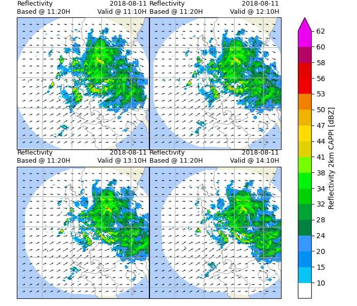
Generating radar reflectivity maps
Define the color scale and format of the plots and plot using xarray.plot().
In this example, only hourly images will be plotted.
# Defining colour scale and format
levels = [
    -32768,
    10, 15, 20, 24, 28, 32,
    34, 38, 41, 44, 47, 50,
    53, 56, 58, 60, 62
]
cmap = ListedColormap([
    '#FFFFFF', '#08C5F5', '#0091F3', '#3898FF', '#008243', '#00A433',
    '#00D100', '#01F508', '#77FF00', '#E0D100', '#FFDC01', '#EEB200',
    '#F08100', '#F00101', '#E20200', '#B40466', '#ED02F0'
])

norm = BoundaryNorm(levels, ncolors=cmap.N, clip=True)

# Defining the crs
crs = area_def.to_cartopy_crs()

# Generating a timelist for every hour
timelist = [
    (basetime + pd.Timedelta(minutes=60*i-10)) for i in range(4)
]

# Obtaining the slice of the xarray to be plotted
da_plot = reflectivity.sel(time=timelist)

# Defining motion quivers
qx = motion.coords['easting'].values[::5]
qy = motion.coords['northing'].values[::5]
qu = motion.values[0, ::5, ::5]
qv = motion.values[1, ::5, ::5]

# Defining coastlines
map_shape_file = os.path.join(DATA_DIR, "shape/rsmc")
ocean_color = np.array([[[178, 208, 254]]], dtype=np.uint8)
land_color = cfeature.COLORS['land']
coastline = cfeature.ShapelyFeature(
    list(shpreader.Reader(map_shape_file).geometries()),
    ccrs.PlateCarree()
)

# Plotting
p = da_plot.plot(
    col='time', col_wrap=2,
    subplot_kws={'projection': crs},
    cbar_kwargs={
        'extend': 'max',
        'ticks': levels[1:],
        'format': '%.3g'
    },
    cmap=cmap,
    norm=norm
)
for idx, ax in enumerate(p.axes.flat):
    # ocean
    ax.imshow(np.tile(ocean_color, [2, 2, 1]),
              origin='upper',
              transform=ccrs.PlateCarree(),
              extent=[-180, 180, -180, 180],
              zorder=-1)
    # coastline, color
    ax.add_feature(coastline,
                   facecolor=land_color, edgecolor='none', zorder=0)
    # overlay coastline without color
    ax.add_feature(coastline, facecolor='none',
                   edgecolor='gray', linewidth=0.5, zorder=3)

    ax.quiver(qx, qy, qu, qv, pivot='mid', regrid_shape=20)
    ax.gridlines()
    ax.set_title(
        "Reflectivity\n"
        f"Based @ {basetime.strftime('%H:%MH')}",
        loc='left',
        fontsize=9
    )
    ax.set_title(
        ''
    )
    ax.set_title(
        f"{basetime.strftime('%Y-%m-%d')} \n"
        f"Valid @ {timelist[idx].strftime('%H:%MH')} ",
        loc='right',
        fontsize=9
    )
plt.savefig(
    os.path.join(
        OUTPUT_DIR,
        "rover-output-map-mn.png"
    ),
    dpi=300
)

radar_image_time = pd.Timestamp.now()
Accumulating hourly rainfall for 3-hour forecast
Hourly accumulated rainfall is calculated every 30 minutes, the first endtime is the basetime i.e. T+0min.
Convert rainrates to rainfalls in 10 mins with to_rainfall_depth().
Accumulate hourly rainfall every 30 minutes using acc_rainfall_depth().
# Convert reflectivity to rainrates
rainfalls = to_rainfall_depth(reflectivity, a=300, b=1.4)

# Converting the coordinates of xarray from start to endtime
rainfalls.coords['time'] = [
    pd.Timestamp(t) + pd.Timedelta(10, 'm')
    for t in rainfalls.coords['time'].values
]
rainfalls.attrs['step_size'] = pd.Timedelta(10, 'm')

# Accumulate hourly rainfall every 30 minutes
acc_rf = acc_rainfall_depth(
    rainfalls,
    basetime,
    basetime+pd.Timedelta(hours=3)
)
acc_rf.attrs['long_name'] = 'Rainfall accumulated over the past 60 minutes'

acc_time = pd.Timestamp.now()
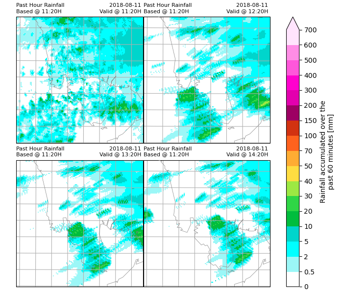
Plotting rainfall maps
Define the colour scheme and format and plot using xarray.plot().
In this example, only hourly images will be plotted.
# Defining the colour scheme
levels = [
    0, 0.5, 2, 5, 10, 20,
    30, 40, 50, 70, 100, 150,
    200, 300, 400, 500, 600, 700
]

cmap = ListedColormap([
    '#ffffff', '#9bf7f7', '#00ffff', '#00d5cc', '#00bd3d', '#2fd646',
    '#9de843', '#ffdd41', '#ffac33', '#ff621e', '#d23211', '#9d0063',
    '#e300ae', '#ff00ce', '#ff57da', '#ff8de6', '#ffe4fd'
])

norm = BoundaryNorm(levels, ncolors=cmap.N, clip=True)

# Defining projection
crs = area_def.to_cartopy_crs()
# Defining zoom extent
r = 64000
proj_site = acc_rf.proj_site
zoom = (
    proj_site[0]-r, proj_site[0]+r, proj_site[1]-r, proj_site[1]+r
)  # (x0, x1, y0, y1)

# Defining times for plotting
timelist = [basetime + pd.Timedelta(i, 'h') for i in range(4)]

# Obtaining xarray slice to be plotted
da_plot = acc_rf.sel(
    easting=slice(zoom[0], zoom[1]),
    northing=slice(zoom[3], zoom[2]),
    time=timelist
)

# Plotting
p = da_plot.plot(
    col='time', col_wrap=2,
    subplot_kws={'projection': crs},
    cbar_kwargs={
        'extend': 'max',
        'ticks': levels,
        'format': '%.3g'
    },
    cmap=cmap,
    norm=norm
)
for idx, ax in enumerate(p.axes.flat):
    # ocean
    ax.imshow(np.tile(ocean_color, [2, 2, 1]),
              origin='upper',
              transform=ccrs.PlateCarree(),
              extent=[-180, 180, -180, 180],
              zorder=-1)
    # coastline, color
    ax.add_feature(coastline,
                   facecolor=land_color, edgecolor='none', zorder=0)
    # overlay coastline without color
    ax.add_feature(coastline, facecolor='none',
                   edgecolor='gray', linewidth=0.5, zorder=3)

    ax.gridlines()
    ax.set_xlim(zoom[0], zoom[1])
    ax.set_ylim(zoom[2], zoom[3])
    ax.set_title(
        "Past Hour Rainfall\n"
        f"Based @ {basetime.strftime('%H:%MH')}",
        loc='left',
        fontsize=8
    )
    ax.set_title(
        ''
    )
    ax.set_title(
        f"{basetime.strftime('%Y-%m-%d')} \n"
        f"Valid @ {timelist[idx].strftime('%H:%MH')} ",
        loc='right',
        fontsize=8
    )
plt.savefig(
    os.path.join(
        OUTPUT_DIR,
        "rainfall_mn.png"
    ),
    dpi=300
)

rf_image_time = pd.Timestamp.now()
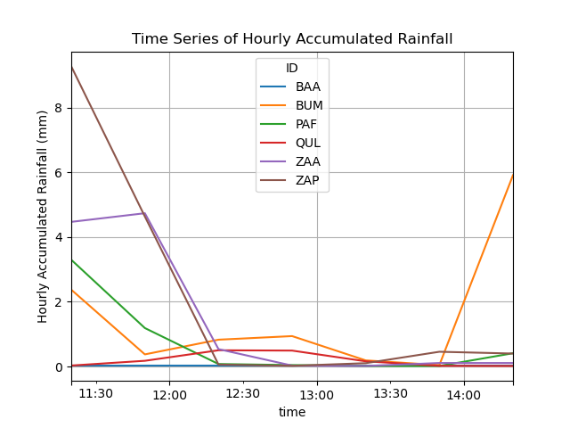
Extract the rainfall values at a specified location
In this example, the rainfall values at the location is assumed to be the same as the nearest gridpoint.
Read information regarding the rain gauge stations into a pandas.DataFrame.
Extract the rainfall values at the nearest gridpoint to location for given timesteps (in this example, 30 minute intervals).
Store rainfall values over time in a pandas.DataFrame.
Plot the time series of rainfall at different stations.
# Getting rain gauge station coordinates
df = pd.read_csv(
    os.path.join(DATA_DIR, "manila_rg_list.csv"),
    delim_whitespace=True,
    usecols=[0, 3, 4]
)

# Extract rainfall values at gridpoint closest to the
# location specified for given timesteps and storing it
# in pandas.DataFrame.

rf_time = []
for time in acc_rf.coords['time'].values:
    rf = []
    for index, row in df.iterrows():
        rf.append(acc_rf.sel(
            time=time, northing=row[2],
            easting=row[1],
            method='nearest'
        ).values)
    rf_time.append(rf)

rf_time = np.array(rf_time)

station_rf = pd.DataFrame(
    data=rf_time,
    columns=df.iloc[:, 0],
    index=pd.Index(
        acc_rf.coords['time'].values,
        name='time'
    )
)

print(station_rf)

loc_stn = ['BAA', 'BUM', 'PAF', 'QUL', 'ZAP', 'ZAA']
loc_stn_drop = [
    stn for stn in station_rf.columns.to_list()
    if stn not in loc_stn
]
df_loc = station_rf.drop(loc_stn_drop, axis=1)

print(df_loc)

# Plotting time series graph for selected stations
ax = df_loc.plot(title="Time Series of Hourly Accumulated Rainfall",
                 grid=True)
ax.set_ylabel("Hourly Accumulated Rainfall (mm)")
plt.savefig(os.path.join(OUTPUT_DIR, "qpf_time_series.png"))

extract_time = pd.Timestamp.now()
ID                        BAA       BAL       BAT  ...       ZAB       ZAM       ZAP
time                                               ...
2018-08-11 11:20:00  0.017007  0.223561  0.017007  ...  2.524197  3.811615  9.269530
2018-08-11 11:50:00  0.017007  0.086412  0.017007  ...  0.737381  3.271796  4.631453
2018-08-11 12:20:00  0.017007  0.020272  0.017007  ...  0.282069  0.172685  0.058832
2018-08-11 12:50:00  0.017007  0.017007  0.017007  ...  0.295333  8.135465  0.020994
2018-08-11 13:20:00  0.017007  0.017007  0.017007  ...  0.259161  7.980322  0.102624
2018-08-11 13:50:00  0.017007  0.017007  0.017007  ...  0.206496  0.017542  0.455374
2018-08-11 14:20:00  0.017007  0.017007  0.017007  ...  0.114196  0.021589  0.399646

[7 rows x 33 columns]
ID                        BAA       BUM       PAF       QUL       ZAA       ZAP
time
2018-08-11 11:20:00  0.017007  2.371822  3.295300  0.029450  4.466178  9.269530
2018-08-11 11:50:00  0.017007  0.374256  1.187007  0.175955  4.733512  4.631453
2018-08-11 12:20:00  0.017007  0.827810  0.076416  0.500572  0.535865  0.058832
2018-08-11 12:50:00  0.017007  0.938581  0.043591  0.491115  0.027811  0.020994
2018-08-11 13:20:00  0.017007  0.188063  0.017007  0.160100  0.017007  0.102624
2018-08-11 13:50:00  0.017007  0.043969  0.017007  0.020873  0.107931  0.455374
2018-08-11 14:20:00  0.017007  5.908081  0.409321  0.017007  0.107931  0.399646
Checking run time of each component
print(f"Start time: {start_time}")
print(f"Initialising time: {initialising_time}")
print(f"Rover time: {rover_time}")
print(f"SLA time: {sla_time}")
print(f"Plotting radar image time: {radar_image_time}")
print(f"Accumulating rainfall time: {acc_time}")
print(f"Concatenating time: {concat_time}")
print(f"Plotting rainfall map time: {rf_image_time}")
print(f"Extracting and plotting time series time: {extract_time}")

print(f"Time to initialise: {initialising_time-start_time}")
print(f"Time to run rover: {rover_time-initialising_time}")
print(f"Time to perform SLA: {sla_time-rover_time}")
print(f"Time to concatenate xarrays: {concat_time - sla_time}")
print(f"Time to plot radar image: {radar_image_time - concat_time}")
print(f"Time to accumulate rainfall: {acc_time - radar_image_time}")
print(f"Time to plot rainfall maps: {rf_image_time-acc_time}")
print(f"Time to extract and plot time series: {extract_time-rf_image_time}")
Start time: 2026-04-20 20:32:59.848764
Initialising time: 2026-04-20 20:33:38.422581
Rover time: 2026-04-20 20:33:38.512821
SLA time: 2026-04-20 20:33:51.108216
Plotting radar image time: 2026-04-20 20:34:22.093591
Accumulating rainfall time: 2026-04-20 20:34:24.606160
Concatenating time: 2026-04-20 20:33:51.154656
Plotting rainfall map time: 2026-04-20 20:34:31.063831
Extracting and plotting time series time: 2026-04-20 20:34:33.780184
Time to initialise: 0 days 00:00:38.573817
Time to run rover: 0 days 00:00:00.090240
Time to perform SLA: 0 days 00:00:12.595395
Time to concatenate xarrays: 0 days 00:00:00.046440
Time to plot radar image: 0 days 00:00:30.938935
Time to accumulate rainfall: 0 days 00:00:02.512569
Time to plot rainfall maps: 0 days 00:00:06.457671
Time to extract and plot time series: 0 days 00:00:02.716353
Total running time of the script: ( 1 minutes 33.998 seconds)