Note
Click here to download the full example code
TrajGRU (Hong Kong)
This example demonstrates how to use pre-trained TrajGRU model to predict the next two-hour forecast using thirty-minute radar echo maps.
Definitions
Import all required modules and methods:
# Python package to allow system command line functions
import os
# Python package to manage warning message
import warnings
# Python package for datetime function
import datetime
# Python package for xarrays to read and handle netcdf data
import xarray as xr
# Python package for ndarray operations
import numpy as np
# Python package for projection description
from pyresample.geometry import AreaDefinition
from pyresample import get_area_def
# Python package for projection
import cartopy.crs as ccrs
# Python package for land/sea features
import cartopy.feature as cfeature
# Python package for reading map shape file
import cartopy.io.shapereader as shpreader
# Python package for creating plots
from matplotlib import pyplot as plt
# Python package for colorbars
from matplotlib.colors import BoundaryNorm, ListedColormap
# swirlspy regrid function
from swirlspy.core.resample import grid_resample
# swirlspy standardize data function
from swirlspy.utils import standardize_attr, FrameType
# swirlspy cuda checking function
from swirlspy.utils import locate_cuda
# swirlspy deep learning function
from swirlspy.qpf.dl.config import cfg
from swirlspy.qpf.dl.hko_benchmark import HKOBenchmarkEnv
from swirlspy.qpf.dl.hko_evaluation import pixel_to_dBZ
# directory constants
from swirlspy.tests.samples import DATA_DIR
from swirlspy.tests.outputs import OUTPUT_DIR
from swirlspy.tests.models import DL_MODEL_DIR
from swirlspy.qpf.dl.models.trajgru.predictor import TrajgruNowcastPredictor

warnings.filterwarnings("ignore")
Initialising
This section demonstrates the settings to run the pre-trained model.
# use GPU if CUDA installed; otherwise use CPU
if locate_cuda():
    ctx = 'gpu'
else:
    ctx = 'cpu'

# Initialize the Trajgru Nowcast Predictor with Pre-trained model
predictor = TrajgruNowcastPredictor(device=ctx)
base_dir = os.path.join(DL_MODEL_DIR, 'hko/%s' % (predictor.name,))

# no training on inference data: mode = 'fixed' and finetune = 0
# train on inference data: mode = 'online' and finetune = 1
mode = 'fixed'
finetune = 0

# 2019-04-20 10:30 to 2019-04-20 15:24
pd_path = cfg.HKO_PD.RAINY_EXAMPLE

# Set the save directory
save_dir = os.path.join(base_dir, "iter%d_%s_finetune%d"
                        % (cfg.MODEL.LOAD_ITER + 1, 'example',
                           finetune))

# Create the environment to run the model
env = HKOBenchmarkEnv(pd_path=pd_path, save_dir=save_dir, mode=mode)
Downloading data from http://swirlsgpu01/data/swirlspy/models/trajgru/v2/encoder_forecaster_100000.pth

Downloading: [--------------------------------------------------] 0%
Downloading: [--------------------------------------------------] 0%
Downloading: [--------------------------------------------------] 0%
Downloading: [--------------------------------------------------] 0%
Downloading: [--------------------------------------------------] 0%
Downloading: [--------------------------------------------------] 0%
Downloading: [--------------------------------------------------] 0%
Downloading: [--------------------------------------------------] 0%
Downloading: [--------------------------------------------------] 0%
Downloading: [--------------------------------------------------] 0%
Downloading: [--------------------------------------------------] 0%
Downloading: [--------------------------------------------------] 0%
Downloading: [--------------------------------------------------] 0%
Downloading: [--------------------------------------------------] 0%
Downloading: [--------------------------------------------------] 0%
Downloading: [--------------------------------------------------] 0%
Downloading: [--------------------------------------------------] 0%
Downloading: [--------------------------------------------------] 0%
Downloading: [--------------------------------------------------] 0%
Downloading: [--------------------------------------------------] 0%
Downloading: [--------------------------------------------------] 0%
Downloading: [--------------------------------------------------] 0%
Downloading: [--------------------------------------------------] 0%
Downloading: [--------------------------------------------------] 0%
Downloading: [--------------------------------------------------] 0%
Downloading: [--------------------------------------------------] 0%
Downloading: [--------------------------------------------------] 0%
Downloading: [--------------------------------------------------] 0%
Downloading: [--------------------------------------------------] 0%
Downloading: [--------------------------------------------------] 0%
Downloading: [--------------------------------------------------] 0%
Downloading: [--------------------------------------------------] 0%
Downloading: [--------------------------------------------------] 0%
Downloading: [--------------------------------------------------] 0%
Downloading: [--------------------------------------------------] 0%
Downloading: [--------------------------------------------------] 0%
Downloading: [--------------------------------------------------] 0%
Downloading: [--------------------------------------------------] 0%
Downloading: [--------------------------------------------------] 0%
Downloading: [--------------------------------------------------] 0%
Downloading: [--------------------------------------------------] 0%
Downloading: [--------------------------------------------------] 0%
Downloading: [--------------------------------------------------] 0%
Downloading: [--------------------------------------------------] 0%
Downloading: [--------------------------------------------------] 0%
Downloading: [--------------------------------------------------] 0%
Downloading: [--------------------------------------------------] 0%
Downloading: [--------------------------------------------------] 0%
Downloading: [--------------------------------------------------] 0%
Downloading: [--------------------------------------------------] 0%
Downloading: [--------------------------------------------------] 0%
Downloading: [--------------------------------------------------] 0%
Downloading: [--------------------------------------------------] 0%
Downloading: [--------------------------------------------------] 0%
Downloading: [--------------------------------------------------] 0%
Downloading: [--------------------------------------------------] 0%
Downloading: [--------------------------------------------------] 0%
Downloading: [--------------------------------------------------] 0%
Downloading: [--------------------------------------------------] 0%
Downloading: [--------------------------------------------------] 0%
Downloading: [--------------------------------------------------] 0%
Downloading: [--------------------------------------------------] 0%
Downloading: [--------------------------------------------------] 0%
Downloading: [--------------------------------------------------] 1%
Downloading: [--------------------------------------------------] 1%
Downloading: [--------------------------------------------------] 1%
Downloading: [--------------------------------------------------] 1%
Downloading: [--------------------------------------------------] 1%
Downloading: [--------------------------------------------------] 1%
Downloading: [--------------------------------------------------] 1%
Downloading: [--------------------------------------------------] 1%
Downloading: [--------------------------------------------------] 1%
Downloading: [--------------------------------------------------] 1%
Downloading: [--------------------------------------------------] 1%
Downloading: [--------------------------------------------------] 1%
Downloading: [--------------------------------------------------] 1%
Downloading: [--------------------------------------------------] 1%
Downloading: [--------------------------------------------------] 1%
Downloading: [--------------------------------------------------] 1%
Downloading: [--------------------------------------------------] 1%
Downloading: [--------------------------------------------------] 1%
Downloading: [--------------------------------------------------] 1%
Downloading: [--------------------------------------------------] 1%
Downloading: [--------------------------------------------------] 1%
Downloading: [--------------------------------------------------] 1%
Downloading: [--------------------------------------------------] 1%
Downloading: [--------------------------------------------------] 1%
Downloading: [--------------------------------------------------] 1%
Downloading: [--------------------------------------------------] 1%
Downloading: [--------------------------------------------------] 1%
Downloading: [--------------------------------------------------] 1%
Downloading: [--------------------------------------------------] 1%
Downloading: [--------------------------------------------------] 1%
Downloading: [--------------------------------------------------] 1%
Downloading: [--------------------------------------------------] 1%
Downloading: [--------------------------------------------------] 1%
Downloading: [--------------------------------------------------] 1%
Downloading: [--------------------------------------------------] 1%
Downloading: [--------------------------------------------------] 1%
Downloading: [--------------------------------------------------] 1%
Downloading: [--------------------------------------------------] 1%
Downloading: [--------------------------------------------------] 1%
Downloading: [--------------------------------------------------] 1%
Downloading: [--------------------------------------------------] 1%
Downloading: [--------------------------------------------------] 1%
Downloading: [--------------------------------------------------] 1%
Downloading: [--------------------------------------------------] 1%
Downloading: [--------------------------------------------------] 1%
Downloading: [--------------------------------------------------] 1%
Downloading: [--------------------------------------------------] 1%
Downloading: [--------------------------------------------------] 1%
Downloading: [--------------------------------------------------] 1%
Downloading: [--------------------------------------------------] 1%
Downloading: [--------------------------------------------------] 1%
Downloading: [--------------------------------------------------] 1%
Downloading: [--------------------------------------------------] 1%
Downloading: [--------------------------------------------------] 1%
Downloading: [--------------------------------------------------] 1%
Downloading: [--------------------------------------------------] 1%
Downloading: [--------------------------------------------------] 1%
Downloading: [--------------------------------------------------] 1%
Downloading: [--------------------------------------------------] 1%
Downloading: [--------------------------------------------------] 1%
Downloading: [--------------------------------------------------] 1%
Downloading: [--------------------------------------------------] 1%
Downloading: [#-------------------------------------------------] 2%
Downloading: [#-------------------------------------------------] 2%
Downloading: [#-------------------------------------------------] 2%
Downloading: [#-------------------------------------------------] 2%
Downloading: [#-------------------------------------------------] 2%
Downloading: [#-------------------------------------------------] 2%
Downloading: [#-------------------------------------------------] 2%
Downloading: [#-------------------------------------------------] 2%
Downloading: [#-------------------------------------------------] 2%
Downloading: [#-------------------------------------------------] 2%
Downloading: [#-------------------------------------------------] 2%
Downloading: [#-------------------------------------------------] 2%
Downloading: [#-------------------------------------------------] 2%
Downloading: [#-------------------------------------------------] 2%
Downloading: [#-------------------------------------------------] 2%
Downloading: [#-------------------------------------------------] 2%
Downloading: [#-------------------------------------------------] 2%
Downloading: [#-------------------------------------------------] 2%
Downloading: [#-------------------------------------------------] 2%
Downloading: [#-------------------------------------------------] 2%
Downloading: [#-------------------------------------------------] 2%
Downloading: [#-------------------------------------------------] 2%
Downloading: [#-------------------------------------------------] 2%
Downloading: [#-------------------------------------------------] 2%
Downloading: [#-------------------------------------------------] 2%
Downloading: [#-------------------------------------------------] 2%
Downloading: [#-------------------------------------------------] 2%
Downloading: [#-------------------------------------------------] 2%
Downloading: [#-------------------------------------------------] 2%
Downloading: [#-------------------------------------------------] 2%
Downloading: [#-------------------------------------------------] 2%
Downloading: [#-------------------------------------------------] 2%
Downloading: [#-------------------------------------------------] 2%
Downloading: [#-------------------------------------------------] 2%
Downloading: [#-------------------------------------------------] 2%
Downloading: [#-------------------------------------------------] 2%
Downloading: [#-------------------------------------------------] 2%
Downloading: [#-------------------------------------------------] 2%
Downloading: [#-------------------------------------------------] 2%
Downloading: [#-------------------------------------------------] 2%
Downloading: [#-------------------------------------------------] 2%
Downloading: [#-------------------------------------------------] 2%
Downloading: [#-------------------------------------------------] 2%
Downloading: [#-------------------------------------------------] 2%
Downloading: [#-------------------------------------------------] 2%
Downloading: [#-------------------------------------------------] 2%
Downloading: [#-------------------------------------------------] 2%
Downloading: [#-------------------------------------------------] 2%
Downloading: [#-------------------------------------------------] 2%
Downloading: [#-------------------------------------------------] 2%
Downloading: [#-------------------------------------------------] 2%
Downloading: [#-------------------------------------------------] 2%
Downloading: [#-------------------------------------------------] 2%
Downloading: [#-------------------------------------------------] 2%
Downloading: [#-------------------------------------------------] 2%
Downloading: [#-------------------------------------------------] 2%
Downloading: [#-------------------------------------------------] 2%
Downloading: [#-------------------------------------------------] 2%
Downloading: [#-------------------------------------------------] 2%
Downloading: [#-------------------------------------------------] 2%
Downloading: [#-------------------------------------------------] 2%
Downloading: [#-------------------------------------------------] 2%
Downloading: [#-------------------------------------------------] 3%
Downloading: [#-------------------------------------------------] 3%
Downloading: [#-------------------------------------------------] 3%
Downloading: [#-------------------------------------------------] 3%
Downloading: [#-------------------------------------------------] 3%
Downloading: [#-------------------------------------------------] 3%
Downloading: [#-------------------------------------------------] 3%
Downloading: [#-------------------------------------------------] 3%
Downloading: [#-------------------------------------------------] 3%
Downloading: [#-------------------------------------------------] 3%
Downloading: [#-------------------------------------------------] 3%
Downloading: [#-------------------------------------------------] 3%
Downloading: [#-------------------------------------------------] 3%
Downloading: [#-------------------------------------------------] 3%
Downloading: [#-------------------------------------------------] 3%
Downloading: [#-------------------------------------------------] 3%
Downloading: [#-------------------------------------------------] 3%
Downloading: [#-------------------------------------------------] 3%
Downloading: [#-------------------------------------------------] 3%
Downloading: [#-------------------------------------------------] 3%
Downloading: [#-------------------------------------------------] 3%
Downloading: [#-------------------------------------------------] 3%
Downloading: [#-------------------------------------------------] 3%
Downloading: [#-------------------------------------------------] 3%
Downloading: [#-------------------------------------------------] 3%
Downloading: [#-------------------------------------------------] 3%
Downloading: [#-------------------------------------------------] 3%
Downloading: [#-------------------------------------------------] 3%
Downloading: [#-------------------------------------------------] 3%
Downloading: [#-------------------------------------------------] 3%
Downloading: [#-------------------------------------------------] 3%
Downloading: [#-------------------------------------------------] 3%
Downloading: [#-------------------------------------------------] 3%
Downloading: [#-------------------------------------------------] 3%
Downloading: [#-------------------------------------------------] 3%
Downloading: [#-------------------------------------------------] 3%
Downloading: [#-------------------------------------------------] 3%
Downloading: [#-------------------------------------------------] 3%
Downloading: [#-------------------------------------------------] 3%
Downloading: [#-------------------------------------------------] 3%
Downloading: [#-------------------------------------------------] 3%
Downloading: [#-------------------------------------------------] 3%
Downloading: [#-------------------------------------------------] 3%
Downloading: [#-------------------------------------------------] 3%
Downloading: [#-------------------------------------------------] 3%
Downloading: [#-------------------------------------------------] 3%
Downloading: [#-------------------------------------------------] 3%
Downloading: [#-------------------------------------------------] 3%
Downloading: [#-------------------------------------------------] 3%
Downloading: [#-------------------------------------------------] 3%
Downloading: [#-------------------------------------------------] 3%
Downloading: [#-------------------------------------------------] 3%
Downloading: [#-------------------------------------------------] 3%
Downloading: [#-------------------------------------------------] 3%
Downloading: [#-------------------------------------------------] 3%
Downloading: [#-------------------------------------------------] 3%
Downloading: [#-------------------------------------------------] 3%
Downloading: [#-------------------------------------------------] 3%
Downloading: [#-------------------------------------------------] 3%
Downloading: [#-------------------------------------------------] 3%
Downloading: [#-------------------------------------------------] 3%
Downloading: [#-------------------------------------------------] 3%
Downloading: [#-------------------------------------------------] 3%
Downloading: [##------------------------------------------------] 4%
Downloading: [##------------------------------------------------] 4%
Downloading: [##------------------------------------------------] 4%
Downloading: [##------------------------------------------------] 4%
Downloading: [##------------------------------------------------] 4%
Downloading: [##------------------------------------------------] 4%
Downloading: [##------------------------------------------------] 4%
Downloading: [##------------------------------------------------] 4%
Downloading: [##------------------------------------------------] 4%
Downloading: [##------------------------------------------------] 4%
Downloading: [##------------------------------------------------] 4%
Downloading: [##------------------------------------------------] 4%
Downloading: [##------------------------------------------------] 4%
Downloading: [##------------------------------------------------] 4%
Downloading: [##------------------------------------------------] 4%
Downloading: [##------------------------------------------------] 4%
Downloading: [##------------------------------------------------] 4%
Downloading: [##------------------------------------------------] 4%
Downloading: [##------------------------------------------------] 4%
Downloading: [##------------------------------------------------] 4%
Downloading: [##------------------------------------------------] 4%
Downloading: [##------------------------------------------------] 4%
Downloading: [##------------------------------------------------] 4%
Downloading: [##------------------------------------------------] 4%
Downloading: [##------------------------------------------------] 4%
Downloading: [##------------------------------------------------] 4%
Downloading: [##------------------------------------------------] 4%
Downloading: [##------------------------------------------------] 4%
Downloading: [##------------------------------------------------] 4%
Downloading: [##------------------------------------------------] 4%
Downloading: [##------------------------------------------------] 4%
Downloading: [##------------------------------------------------] 4%
Downloading: [##------------------------------------------------] 4%
Downloading: [##------------------------------------------------] 4%
Downloading: [##------------------------------------------------] 4%
Downloading: [##------------------------------------------------] 4%
Downloading: [##------------------------------------------------] 4%
Downloading: [##------------------------------------------------] 4%
Downloading: [##------------------------------------------------] 4%
Downloading: [##------------------------------------------------] 4%
Downloading: [##------------------------------------------------] 4%
Downloading: [##------------------------------------------------] 4%
Downloading: [##------------------------------------------------] 4%
Downloading: [##------------------------------------------------] 4%
Downloading: [##------------------------------------------------] 4%
Downloading: [##------------------------------------------------] 4%
Downloading: [##------------------------------------------------] 4%
Downloading: [##------------------------------------------------] 4%
Downloading: [##------------------------------------------------] 4%
Downloading: [##------------------------------------------------] 4%
Downloading: [##------------------------------------------------] 4%
Downloading: [##------------------------------------------------] 4%
Downloading: [##------------------------------------------------] 4%
Downloading: [##------------------------------------------------] 4%
Downloading: [##------------------------------------------------] 4%
Downloading: [##------------------------------------------------] 4%
Downloading: [##------------------------------------------------] 4%
Downloading: [##------------------------------------------------] 4%
Downloading: [##------------------------------------------------] 4%
Downloading: [##------------------------------------------------] 4%
Downloading: [##------------------------------------------------] 4%
Downloading: [##------------------------------------------------] 4%
Downloading: [##------------------------------------------------] 5%
Downloading: [##------------------------------------------------] 5%
Downloading: [##------------------------------------------------] 5%
Downloading: [##------------------------------------------------] 5%
Downloading: [##------------------------------------------------] 5%
Downloading: [##------------------------------------------------] 5%
Downloading: [##------------------------------------------------] 5%
Downloading: [##------------------------------------------------] 5%
Downloading: [##------------------------------------------------] 5%
Downloading: [##------------------------------------------------] 5%
Downloading: [##------------------------------------------------] 5%
Downloading: [##------------------------------------------------] 5%
Downloading: [##------------------------------------------------] 5%
Downloading: [##------------------------------------------------] 5%
Downloading: [##------------------------------------------------] 5%
Downloading: [##------------------------------------------------] 5%
Downloading: [##------------------------------------------------] 5%
Downloading: [##------------------------------------------------] 5%
Downloading: [##------------------------------------------------] 5%
Downloading: [##------------------------------------------------] 5%
Downloading: [##------------------------------------------------] 5%
Downloading: [##------------------------------------------------] 5%
Downloading: [##------------------------------------------------] 5%
Downloading: [##------------------------------------------------] 5%
Downloading: [##------------------------------------------------] 5%
Downloading: [##------------------------------------------------] 5%
Downloading: [##------------------------------------------------] 5%
Downloading: [##------------------------------------------------] 5%
Downloading: [##------------------------------------------------] 5%
Downloading: [##------------------------------------------------] 5%
Downloading: [##------------------------------------------------] 5%
Downloading: [##------------------------------------------------] 5%
Downloading: [##------------------------------------------------] 5%
Downloading: [##------------------------------------------------] 5%
Downloading: [##------------------------------------------------] 5%
Downloading: [##------------------------------------------------] 5%
Downloading: [##------------------------------------------------] 5%
Downloading: [##------------------------------------------------] 5%
Downloading: [##------------------------------------------------] 5%
Downloading: [##------------------------------------------------] 5%
Downloading: [##------------------------------------------------] 5%
Downloading: [##------------------------------------------------] 5%
Downloading: [##------------------------------------------------] 5%
Downloading: [##------------------------------------------------] 5%
Downloading: [##------------------------------------------------] 5%
Downloading: [##------------------------------------------------] 5%
Downloading: [##------------------------------------------------] 5%
Downloading: [##------------------------------------------------] 5%
Downloading: [##------------------------------------------------] 5%
Downloading: [##------------------------------------------------] 5%
Downloading: [##------------------------------------------------] 5%
Downloading: [##------------------------------------------------] 5%
Downloading: [##------------------------------------------------] 5%
Downloading: [##------------------------------------------------] 5%
Downloading: [##------------------------------------------------] 5%
Downloading: [##------------------------------------------------] 5%
Downloading: [##------------------------------------------------] 5%
Downloading: [##------------------------------------------------] 5%
Downloading: [##------------------------------------------------] 5%
Downloading: [##------------------------------------------------] 5%
Downloading: [##------------------------------------------------] 5%
Downloading: [##------------------------------------------------] 5%
Downloading: [###-----------------------------------------------] 6%
Downloading: [###-----------------------------------------------] 6%
Downloading: [###-----------------------------------------------] 6%
Downloading: [###-----------------------------------------------] 6%
Downloading: [###-----------------------------------------------] 6%
Downloading: [###-----------------------------------------------] 6%
Downloading: [###-----------------------------------------------] 6%
Downloading: [###-----------------------------------------------] 6%
Downloading: [###-----------------------------------------------] 6%
Downloading: [###-----------------------------------------------] 6%
Downloading: [###-----------------------------------------------] 6%
Downloading: [###-----------------------------------------------] 6%
Downloading: [###-----------------------------------------------] 6%
Downloading: [###-----------------------------------------------] 6%
Downloading: [###-----------------------------------------------] 6%
Downloading: [###-----------------------------------------------] 6%
Downloading: [###-----------------------------------------------] 6%
Downloading: [###-----------------------------------------------] 6%
Downloading: [###-----------------------------------------------] 6%
Downloading: [###-----------------------------------------------] 6%
Downloading: [###-----------------------------------------------] 6%
Downloading: [###-----------------------------------------------] 6%
Downloading: [###-----------------------------------------------] 6%
Downloading: [###-----------------------------------------------] 6%
Downloading: [###-----------------------------------------------] 6%
Downloading: [###-----------------------------------------------] 6%
Downloading: [###-----------------------------------------------] 6%
Downloading: [###-----------------------------------------------] 6%
Downloading: [###-----------------------------------------------] 6%
Downloading: [###-----------------------------------------------] 6%
Downloading: [###-----------------------------------------------] 6%
Downloading: [###-----------------------------------------------] 6%
Downloading: [###-----------------------------------------------] 6%
Downloading: [###-----------------------------------------------] 6%
Downloading: [###-----------------------------------------------] 6%
Downloading: [###-----------------------------------------------] 6%
Downloading: [###-----------------------------------------------] 6%
Downloading: [###-----------------------------------------------] 6%
Downloading: [###-----------------------------------------------] 6%
Downloading: [###-----------------------------------------------] 6%
Downloading: [###-----------------------------------------------] 6%
Downloading: [###-----------------------------------------------] 6%
Downloading: [###-----------------------------------------------] 6%
Downloading: [###-----------------------------------------------] 6%
Downloading: [###-----------------------------------------------] 6%
Downloading: [###-----------------------------------------------] 6%
Downloading: [###-----------------------------------------------] 6%
Downloading: [###-----------------------------------------------] 6%
Downloading: [###-----------------------------------------------] 6%
Downloading: [###-----------------------------------------------] 6%
Downloading: [###-----------------------------------------------] 6%
Downloading: [###-----------------------------------------------] 6%
Downloading: [###-----------------------------------------------] 6%
Downloading: [###-----------------------------------------------] 6%
Downloading: [###-----------------------------------------------] 6%
Downloading: [###-----------------------------------------------] 6%
Downloading: [###-----------------------------------------------] 6%
Downloading: [###-----------------------------------------------] 6%
Downloading: [###-----------------------------------------------] 6%
Downloading: [###-----------------------------------------------] 6%
Downloading: [###-----------------------------------------------] 6%
Downloading: [###-----------------------------------------------] 6%
Downloading: [###-----------------------------------------------] 6%
Downloading: [###-----------------------------------------------] 7%
Downloading: [###-----------------------------------------------] 7%
Downloading: [###-----------------------------------------------] 7%
Downloading: [###-----------------------------------------------] 7%
Downloading: [###-----------------------------------------------] 7%
Downloading: [###-----------------------------------------------] 7%
Downloading: [###-----------------------------------------------] 7%
Downloading: [###-----------------------------------------------] 7%
Downloading: [###-----------------------------------------------] 7%
Downloading: [###-----------------------------------------------] 7%
Downloading: [###-----------------------------------------------] 7%
Downloading: [###-----------------------------------------------] 7%
Downloading: [###-----------------------------------------------] 7%
Downloading: [###-----------------------------------------------] 7%
Downloading: [###-----------------------------------------------] 7%
Downloading: [###-----------------------------------------------] 7%
Downloading: [###-----------------------------------------------] 7%
Downloading: [###-----------------------------------------------] 7%
Downloading: [###-----------------------------------------------] 7%
Downloading: [###-----------------------------------------------] 7%
Downloading: [###-----------------------------------------------] 7%
Downloading: [###-----------------------------------------------] 7%
Downloading: [###-----------------------------------------------] 7%
Downloading: [###-----------------------------------------------] 7%
Downloading: [###-----------------------------------------------] 7%
Downloading: [###-----------------------------------------------] 7%
Downloading: [###-----------------------------------------------] 7%
Downloading: [###-----------------------------------------------] 7%
Downloading: [###-----------------------------------------------] 7%
Downloading: [###-----------------------------------------------] 7%
Downloading: [###-----------------------------------------------] 7%
Downloading: [###-----------------------------------------------] 7%
Downloading: [###-----------------------------------------------] 7%
Downloading: [###-----------------------------------------------] 7%
Downloading: [###-----------------------------------------------] 7%
Downloading: [###-----------------------------------------------] 7%
Downloading: [###-----------------------------------------------] 7%
Downloading: [###-----------------------------------------------] 7%
Downloading: [###-----------------------------------------------] 7%
Downloading: [###-----------------------------------------------] 7%
Downloading: [###-----------------------------------------------] 7%
Downloading: [###-----------------------------------------------] 7%
Downloading: [###-----------------------------------------------] 7%
Downloading: [###-----------------------------------------------] 7%
Downloading: [###-----------------------------------------------] 7%
Downloading: [###-----------------------------------------------] 7%
Downloading: [###-----------------------------------------------] 7%
Downloading: [###-----------------------------------------------] 7%
Downloading: [###-----------------------------------------------] 7%
Downloading: [###-----------------------------------------------] 7%
Downloading: [###-----------------------------------------------] 7%
Downloading: [###-----------------------------------------------] 7%
Downloading: [###-----------------------------------------------] 7%
Downloading: [###-----------------------------------------------] 7%
Downloading: [###-----------------------------------------------] 7%
Downloading: [###-----------------------------------------------] 7%
Downloading: [###-----------------------------------------------] 7%
Downloading: [###-----------------------------------------------] 7%
Downloading: [###-----------------------------------------------] 7%
Downloading: [###-----------------------------------------------] 7%
Downloading: [###-----------------------------------------------] 7%
Downloading: [###-----------------------------------------------] 7%
Downloading: [####----------------------------------------------] 8%
Downloading: [####----------------------------------------------] 8%
Downloading: [####----------------------------------------------] 8%
Downloading: [####----------------------------------------------] 8%
Downloading: [####----------------------------------------------] 8%
Downloading: [####----------------------------------------------] 8%
Downloading: [####----------------------------------------------] 8%
Downloading: [####----------------------------------------------] 8%
Downloading: [####----------------------------------------------] 8%
Downloading: [####----------------------------------------------] 8%
Downloading: [####----------------------------------------------] 8%
Downloading: [####----------------------------------------------] 8%
Downloading: [####----------------------------------------------] 8%
Downloading: [####----------------------------------------------] 8%
Downloading: [####----------------------------------------------] 8%
Downloading: [####----------------------------------------------] 8%
Downloading: [####----------------------------------------------] 8%
Downloading: [####----------------------------------------------] 8%
Downloading: [####----------------------------------------------] 8%
Downloading: [####----------------------------------------------] 8%
Downloading: [####----------------------------------------------] 8%
Downloading: [####----------------------------------------------] 8%
Downloading: [####----------------------------------------------] 8%
Downloading: [####----------------------------------------------] 8%
Downloading: [####----------------------------------------------] 8%
Downloading: [####----------------------------------------------] 8%
Downloading: [####----------------------------------------------] 8%
Downloading: [####----------------------------------------------] 8%
Downloading: [####----------------------------------------------] 8%
Downloading: [####----------------------------------------------] 8%
Downloading: [####----------------------------------------------] 8%
Downloading: [####----------------------------------------------] 8%
Downloading: [####----------------------------------------------] 8%
Downloading: [####----------------------------------------------] 8%
Downloading: [####----------------------------------------------] 8%
Downloading: [####----------------------------------------------] 8%
Downloading: [####----------------------------------------------] 8%
Downloading: [####----------------------------------------------] 8%
Downloading: [####----------------------------------------------] 8%
Downloading: [####----------------------------------------------] 8%
Downloading: [####----------------------------------------------] 8%
Downloading: [####----------------------------------------------] 8%
Downloading: [####----------------------------------------------] 8%
Downloading: [####----------------------------------------------] 8%
Downloading: [####----------------------------------------------] 8%
Downloading: [####----------------------------------------------] 8%
Downloading: [####----------------------------------------------] 8%
Downloading: [####----------------------------------------------] 8%
Downloading: [####----------------------------------------------] 8%
Downloading: [####----------------------------------------------] 8%
Downloading: [####----------------------------------------------] 8%
Downloading: [####----------------------------------------------] 8%
Downloading: [####----------------------------------------------] 8%
Downloading: [####----------------------------------------------] 8%
Downloading: [####----------------------------------------------] 8%
Downloading: [####----------------------------------------------] 8%
Downloading: [####----------------------------------------------] 8%
Downloading: [####----------------------------------------------] 8%
Downloading: [####----------------------------------------------] 8%
Downloading: [####----------------------------------------------] 8%
Downloading: [####----------------------------------------------] 8%
Downloading: [####----------------------------------------------] 8%
Downloading: [####----------------------------------------------] 9%
Downloading: [####----------------------------------------------] 9%
Downloading: [####----------------------------------------------] 9%
Downloading: [####----------------------------------------------] 9%
Downloading: [####----------------------------------------------] 9%
Downloading: [####----------------------------------------------] 9%
Downloading: [####----------------------------------------------] 9%
Downloading: [####----------------------------------------------] 9%
Downloading: [####----------------------------------------------] 9%
Downloading: [####----------------------------------------------] 9%
Downloading: [####----------------------------------------------] 9%
Downloading: [####----------------------------------------------] 9%
Downloading: [####----------------------------------------------] 9%
Downloading: [####----------------------------------------------] 9%
Downloading: [####----------------------------------------------] 9%
Downloading: [####----------------------------------------------] 9%
Downloading: [####----------------------------------------------] 9%
Downloading: [####----------------------------------------------] 9%
Downloading: [####----------------------------------------------] 9%
Downloading: [####----------------------------------------------] 9%
Downloading: [####----------------------------------------------] 9%
Downloading: [####----------------------------------------------] 9%
Downloading: [####----------------------------------------------] 9%
Downloading: [####----------------------------------------------] 9%
Downloading: [####----------------------------------------------] 9%
Downloading: [####----------------------------------------------] 9%
Downloading: [####----------------------------------------------] 9%
Downloading: [####----------------------------------------------] 9%
Downloading: [####----------------------------------------------] 9%
Downloading: [####----------------------------------------------] 9%
Downloading: [####----------------------------------------------] 9%
Downloading: [####----------------------------------------------] 9%
Downloading: [####----------------------------------------------] 9%
Downloading: [####----------------------------------------------] 9%
Downloading: [####----------------------------------------------] 9%
Downloading: [####----------------------------------------------] 9%
Downloading: [####----------------------------------------------] 9%
Downloading: [####----------------------------------------------] 9%
Downloading: [####----------------------------------------------] 9%
Downloading: [####----------------------------------------------] 9%
Downloading: [####----------------------------------------------] 9%
Downloading: [####----------------------------------------------] 9%
Downloading: [####----------------------------------------------] 9%
Downloading: [####----------------------------------------------] 9%
Downloading: [####----------------------------------------------] 9%
Downloading: [####----------------------------------------------] 9%
Downloading: [####----------------------------------------------] 9%
Downloading: [####----------------------------------------------] 9%
Downloading: [####----------------------------------------------] 9%
Downloading: [####----------------------------------------------] 9%
Downloading: [####----------------------------------------------] 9%
Downloading: [####----------------------------------------------] 9%
Downloading: [####----------------------------------------------] 9%
Downloading: [####----------------------------------------------] 9%
Downloading: [####----------------------------------------------] 9%
Downloading: [####----------------------------------------------] 9%
Downloading: [####----------------------------------------------] 9%
Downloading: [####----------------------------------------------] 9%
Downloading: [####----------------------------------------------] 9%
Downloading: [####----------------------------------------------] 9%
Downloading: [####----------------------------------------------] 9%
Downloading: [####----------------------------------------------] 9%
Downloading: [####----------------------------------------------] 9%
Downloading: [#####---------------------------------------------] 10%
Downloading: [#####---------------------------------------------] 10%
Downloading: [#####---------------------------------------------] 10%
Downloading: [#####---------------------------------------------] 10%
Downloading: [#####---------------------------------------------] 10%
Downloading: [#####---------------------------------------------] 10%
Downloading: [#####---------------------------------------------] 10%
Downloading: [#####---------------------------------------------] 10%
Downloading: [#####---------------------------------------------] 10%
Downloading: [#####---------------------------------------------] 10%
Downloading: [#####---------------------------------------------] 10%
Downloading: [#####---------------------------------------------] 10%
Downloading: [#####---------------------------------------------] 10%
Downloading: [#####---------------------------------------------] 10%
Downloading: [#####---------------------------------------------] 10%
Downloading: [#####---------------------------------------------] 10%
Downloading: [#####---------------------------------------------] 10%
Downloading: [#####---------------------------------------------] 10%
Downloading: [#####---------------------------------------------] 10%
Downloading: [#####---------------------------------------------] 10%
Downloading: [#####---------------------------------------------] 10%
Downloading: [#####---------------------------------------------] 10%
Downloading: [#####---------------------------------------------] 10%
Downloading: [#####---------------------------------------------] 10%
Downloading: [#####---------------------------------------------] 10%
Downloading: [#####---------------------------------------------] 10%
Downloading: [#####---------------------------------------------] 10%
Downloading: [#####---------------------------------------------] 10%
Downloading: [#####---------------------------------------------] 10%
Downloading: [#####---------------------------------------------] 10%
Downloading: [#####---------------------------------------------] 10%
Downloading: [#####---------------------------------------------] 10%
Downloading: [#####---------------------------------------------] 10%
Downloading: [#####---------------------------------------------] 10%
Downloading: [#####---------------------------------------------] 10%
Downloading: [#####---------------------------------------------] 10%
Downloading: [#####---------------------------------------------] 10%
Downloading: [#####---------------------------------------------] 10%
Downloading: [#####---------------------------------------------] 10%
Downloading: [#####---------------------------------------------] 10%
Downloading: [#####---------------------------------------------] 10%
Downloading: [#####---------------------------------------------] 10%
Downloading: [#####---------------------------------------------] 10%
Downloading: [#####---------------------------------------------] 10%
Downloading: [#####---------------------------------------------] 10%
Downloading: [#####---------------------------------------------] 10%
Downloading: [#####---------------------------------------------] 10%
Downloading: [#####---------------------------------------------] 10%
Downloading: [#####---------------------------------------------] 10%
Downloading: [#####---------------------------------------------] 10%
Downloading: [#####---------------------------------------------] 10%
Downloading: [#####---------------------------------------------] 10%
Downloading: [#####---------------------------------------------] 10%
Downloading: [#####---------------------------------------------] 10%
Downloading: [#####---------------------------------------------] 10%
Downloading: [#####---------------------------------------------] 10%
Downloading: [#####---------------------------------------------] 10%
Downloading: [#####---------------------------------------------] 10%
Downloading: [#####---------------------------------------------] 10%
Downloading: [#####---------------------------------------------] 10%
Downloading: [#####---------------------------------------------] 10%
Downloading: [#####---------------------------------------------] 10%
Downloading: [#####---------------------------------------------] 11%
Downloading: [#####---------------------------------------------] 11%
Downloading: [#####---------------------------------------------] 11%
Downloading: [#####---------------------------------------------] 11%
Downloading: [#####---------------------------------------------] 11%
Downloading: [#####---------------------------------------------] 11%
Downloading: [#####---------------------------------------------] 11%
Downloading: [#####---------------------------------------------] 11%
Downloading: [#####---------------------------------------------] 11%
Downloading: [#####---------------------------------------------] 11%
Downloading: [#####---------------------------------------------] 11%
Downloading: [#####---------------------------------------------] 11%
Downloading: [#####---------------------------------------------] 11%
Downloading: [#####---------------------------------------------] 11%
Downloading: [#####---------------------------------------------] 11%
Downloading: [#####---------------------------------------------] 11%
Downloading: [#####---------------------------------------------] 11%
Downloading: [#####---------------------------------------------] 11%
Downloading: [#####---------------------------------------------] 11%
Downloading: [#####---------------------------------------------] 11%
Downloading: [#####---------------------------------------------] 11%
Downloading: [#####---------------------------------------------] 11%
Downloading: [#####---------------------------------------------] 11%
Downloading: [#####---------------------------------------------] 11%
Downloading: [#####---------------------------------------------] 11%
Downloading: [#####---------------------------------------------] 11%
Downloading: [#####---------------------------------------------] 11%
Downloading: [#####---------------------------------------------] 11%
Downloading: [#####---------------------------------------------] 11%
Downloading: [#####---------------------------------------------] 11%
Downloading: [#####---------------------------------------------] 11%
Downloading: [#####---------------------------------------------] 11%
Downloading: [#####---------------------------------------------] 11%
Downloading: [#####---------------------------------------------] 11%
Downloading: [#####---------------------------------------------] 11%
Downloading: [#####---------------------------------------------] 11%
Downloading: [#####---------------------------------------------] 11%
Downloading: [#####---------------------------------------------] 11%
Downloading: [#####---------------------------------------------] 11%
Downloading: [#####---------------------------------------------] 11%
Downloading: [#####---------------------------------------------] 11%
Downloading: [#####---------------------------------------------] 11%
Downloading: [#####---------------------------------------------] 11%
Downloading: [#####---------------------------------------------] 11%
Downloading: [#####---------------------------------------------] 11%
Downloading: [#####---------------------------------------------] 11%
Downloading: [#####---------------------------------------------] 11%
Downloading: [#####---------------------------------------------] 11%
Downloading: [#####---------------------------------------------] 11%
Downloading: [#####---------------------------------------------] 11%
Downloading: [#####---------------------------------------------] 11%
Downloading: [#####---------------------------------------------] 11%
Downloading: [#####---------------------------------------------] 11%
Downloading: [#####---------------------------------------------] 11%
Downloading: [#####---------------------------------------------] 11%
Downloading: [#####---------------------------------------------] 11%
Downloading: [#####---------------------------------------------] 11%
Downloading: [#####---------------------------------------------] 11%
Downloading: [#####---------------------------------------------] 11%
Downloading: [#####---------------------------------------------] 11%
Downloading: [#####---------------------------------------------] 11%
Downloading: [#####---------------------------------------------] 11%
Downloading: [######--------------------------------------------] 12%
Downloading: [######--------------------------------------------] 12%
Downloading: [######--------------------------------------------] 12%
Downloading: [######--------------------------------------------] 12%
Downloading: [######--------------------------------------------] 12%
Downloading: [######--------------------------------------------] 12%
Downloading: [######--------------------------------------------] 12%
Downloading: [######--------------------------------------------] 12%
Downloading: [######--------------------------------------------] 12%
Downloading: [######--------------------------------------------] 12%
Downloading: [######--------------------------------------------] 12%
Downloading: [######--------------------------------------------] 12%
Downloading: [######--------------------------------------------] 12%
Downloading: [######--------------------------------------------] 12%
Downloading: [######--------------------------------------------] 12%
Downloading: [######--------------------------------------------] 12%
Downloading: [######--------------------------------------------] 12%
Downloading: [######--------------------------------------------] 12%
Downloading: [######--------------------------------------------] 12%
Downloading: [######--------------------------------------------] 12%
Downloading: [######--------------------------------------------] 12%
Downloading: [######--------------------------------------------] 12%
Downloading: [######--------------------------------------------] 12%
Downloading: [######--------------------------------------------] 12%
Downloading: [######--------------------------------------------] 12%
Downloading: [######--------------------------------------------] 12%
Downloading: [######--------------------------------------------] 12%
Downloading: [######--------------------------------------------] 12%
Downloading: [######--------------------------------------------] 12%
Downloading: [######--------------------------------------------] 12%
Downloading: [######--------------------------------------------] 12%
Downloading: [######--------------------------------------------] 12%
Downloading: [######--------------------------------------------] 12%
Downloading: [######--------------------------------------------] 12%
Downloading: [######--------------------------------------------] 12%
Downloading: [######--------------------------------------------] 12%
Downloading: [######--------------------------------------------] 12%
Downloading: [######--------------------------------------------] 12%
Downloading: [######--------------------------------------------] 12%
Downloading: [######--------------------------------------------] 12%
Downloading: [######--------------------------------------------] 12%
Downloading: [######--------------------------------------------] 12%
Downloading: [######--------------------------------------------] 12%
Downloading: [######--------------------------------------------] 12%
Downloading: [######--------------------------------------------] 12%
Downloading: [######--------------------------------------------] 12%
Downloading: [######--------------------------------------------] 12%
Downloading: [######--------------------------------------------] 12%
Downloading: [######--------------------------------------------] 12%
Downloading: [######--------------------------------------------] 12%
Downloading: [######--------------------------------------------] 12%
Downloading: [######--------------------------------------------] 12%
Downloading: [######--------------------------------------------] 12%
Downloading: [######--------------------------------------------] 12%
Downloading: [######--------------------------------------------] 12%
Downloading: [######--------------------------------------------] 12%
Downloading: [######--------------------------------------------] 12%
Downloading: [######--------------------------------------------] 12%
Downloading: [######--------------------------------------------] 12%
Downloading: [######--------------------------------------------] 12%
Downloading: [######--------------------------------------------] 12%
Downloading: [######--------------------------------------------] 12%
Downloading: [######--------------------------------------------] 13%
Downloading: [######--------------------------------------------] 13%
Downloading: [######--------------------------------------------] 13%
Downloading: [######--------------------------------------------] 13%
Downloading: [######--------------------------------------------] 13%
Downloading: [######--------------------------------------------] 13%
Downloading: [######--------------------------------------------] 13%
Downloading: [######--------------------------------------------] 13%
Downloading: [######--------------------------------------------] 13%
Downloading: [######--------------------------------------------] 13%
Downloading: [######--------------------------------------------] 13%
Downloading: [######--------------------------------------------] 13%
Downloading: [######--------------------------------------------] 13%
Downloading: [######--------------------------------------------] 13%
Downloading: [######--------------------------------------------] 13%
Downloading: [######--------------------------------------------] 13%
Downloading: [######--------------------------------------------] 13%
Downloading: [######--------------------------------------------] 13%
Downloading: [######--------------------------------------------] 13%
Downloading: [######--------------------------------------------] 13%
Downloading: [######--------------------------------------------] 13%
Downloading: [######--------------------------------------------] 13%
Downloading: [######--------------------------------------------] 13%
Downloading: [######--------------------------------------------] 13%
Downloading: [######--------------------------------------------] 13%
Downloading: [######--------------------------------------------] 13%
Downloading: [######--------------------------------------------] 13%
Downloading: [######--------------------------------------------] 13%
Downloading: [######--------------------------------------------] 13%
Downloading: [######--------------------------------------------] 13%
Downloading: [######--------------------------------------------] 13%
Downloading: [######--------------------------------------------] 13%
Downloading: [######--------------------------------------------] 13%
Downloading: [######--------------------------------------------] 13%
Downloading: [######--------------------------------------------] 13%
Downloading: [######--------------------------------------------] 13%
Downloading: [######--------------------------------------------] 13%
Downloading: [######--------------------------------------------] 13%
Downloading: [######--------------------------------------------] 13%
Downloading: [######--------------------------------------------] 13%
Downloading: [######--------------------------------------------] 13%
Downloading: [######--------------------------------------------] 13%
Downloading: [######--------------------------------------------] 13%
Downloading: [######--------------------------------------------] 13%
Downloading: [######--------------------------------------------] 13%
Downloading: [######--------------------------------------------] 13%
Downloading: [######--------------------------------------------] 13%
Downloading: [######--------------------------------------------] 13%
Downloading: [######--------------------------------------------] 13%
Downloading: [######--------------------------------------------] 13%
Downloading: [######--------------------------------------------] 13%
Downloading: [######--------------------------------------------] 13%
Downloading: [######--------------------------------------------] 13%
Downloading: [######--------------------------------------------] 13%
Downloading: [######--------------------------------------------] 13%
Downloading: [######--------------------------------------------] 13%
Downloading: [######--------------------------------------------] 13%
Downloading: [######--------------------------------------------] 13%
Downloading: [######--------------------------------------------] 13%
Downloading: [######--------------------------------------------] 13%
Downloading: [######--------------------------------------------] 13%
Downloading: [######--------------------------------------------] 13%
Downloading: [######--------------------------------------------] 13%
Downloading: [#######-------------------------------------------] 14%
Downloading: [#######-------------------------------------------] 14%
Downloading: [#######-------------------------------------------] 14%
Downloading: [#######-------------------------------------------] 14%
Downloading: [#######-------------------------------------------] 14%
Downloading: [#######-------------------------------------------] 14%
Downloading: [#######-------------------------------------------] 14%
Downloading: [#######-------------------------------------------] 14%
Downloading: [#######-------------------------------------------] 14%
Downloading: [#######-------------------------------------------] 14%
Downloading: [#######-------------------------------------------] 14%
Downloading: [#######-------------------------------------------] 14%
Downloading: [#######-------------------------------------------] 14%
Downloading: [#######-------------------------------------------] 14%
Downloading: [#######-------------------------------------------] 14%
Downloading: [#######-------------------------------------------] 14%
Downloading: [#######-------------------------------------------] 14%
Downloading: [#######-------------------------------------------] 14%
Downloading: [#######-------------------------------------------] 14%
Downloading: [#######-------------------------------------------] 14%
Downloading: [#######-------------------------------------------] 14%
Downloading: [#######-------------------------------------------] 14%
Downloading: [#######-------------------------------------------] 14%
Downloading: [#######-------------------------------------------] 14%
Downloading: [#######-------------------------------------------] 14%
Downloading: [#######-------------------------------------------] 14%
Downloading: [#######-------------------------------------------] 14%
Downloading: [#######-------------------------------------------] 14%
Downloading: [#######-------------------------------------------] 14%
Downloading: [#######-------------------------------------------] 14%
Downloading: [#######-------------------------------------------] 14%
Downloading: [#######-------------------------------------------] 14%
Downloading: [#######-------------------------------------------] 14%
Downloading: [#######-------------------------------------------] 14%
Downloading: [#######-------------------------------------------] 14%
Downloading: [#######-------------------------------------------] 14%
Downloading: [#######-------------------------------------------] 14%
Downloading: [#######-------------------------------------------] 14%
Downloading: [#######-------------------------------------------] 14%
Downloading: [#######-------------------------------------------] 14%
Downloading: [#######-------------------------------------------] 14%
Downloading: [#######-------------------------------------------] 14%
Downloading: [#######-------------------------------------------] 14%
Downloading: [#######-------------------------------------------] 14%
Downloading: [#######-------------------------------------------] 14%
Downloading: [#######-------------------------------------------] 14%
Downloading: [#######-------------------------------------------] 14%
Downloading: [#######-------------------------------------------] 14%
Downloading: [#######-------------------------------------------] 14%
Downloading: [#######-------------------------------------------] 14%
Downloading: [#######-------------------------------------------] 14%
Downloading: [#######-------------------------------------------] 14%
Downloading: [#######-------------------------------------------] 14%
Downloading: [#######-------------------------------------------] 14%
Downloading: [#######-------------------------------------------] 14%
Downloading: [#######-------------------------------------------] 14%
Downloading: [#######-------------------------------------------] 14%
Downloading: [#######-------------------------------------------] 14%
Downloading: [#######-------------------------------------------] 14%
Downloading: [#######-------------------------------------------] 14%
Downloading: [#######-------------------------------------------] 14%
Downloading: [#######-------------------------------------------] 14%
Downloading: [#######-------------------------------------------] 15%
Downloading: [#######-------------------------------------------] 15%
Downloading: [#######-------------------------------------------] 15%
Downloading: [#######-------------------------------------------] 15%
Downloading: [#######-------------------------------------------] 15%
Downloading: [#######-------------------------------------------] 15%
Downloading: [#######-------------------------------------------] 15%
Downloading: [#######-------------------------------------------] 15%
Downloading: [#######-------------------------------------------] 15%
Downloading: [#######-------------------------------------------] 15%
Downloading: [#######-------------------------------------------] 15%
Downloading: [#######-------------------------------------------] 15%
Downloading: [#######-------------------------------------------] 15%
Downloading: [#######-------------------------------------------] 15%
Downloading: [#######-------------------------------------------] 15%
Downloading: [#######-------------------------------------------] 15%
Downloading: [#######-------------------------------------------] 15%
Downloading: [#######-------------------------------------------] 15%
Downloading: [#######-------------------------------------------] 15%
Downloading: [#######-------------------------------------------] 15%
Downloading: [#######-------------------------------------------] 15%
Downloading: [#######-------------------------------------------] 15%
Downloading: [#######-------------------------------------------] 15%
Downloading: [#######-------------------------------------------] 15%
Downloading: [#######-------------------------------------------] 15%
Downloading: [#######-------------------------------------------] 15%
Downloading: [#######-------------------------------------------] 15%
Downloading: [#######-------------------------------------------] 15%
Downloading: [#######-------------------------------------------] 15%
Downloading: [#######-------------------------------------------] 15%
Downloading: [#######-------------------------------------------] 15%
Downloading: [#######-------------------------------------------] 15%
Downloading: [#######-------------------------------------------] 15%
Downloading: [#######-------------------------------------------] 15%
Downloading: [#######-------------------------------------------] 15%
Downloading: [#######-------------------------------------------] 15%
Downloading: [#######-------------------------------------------] 15%
Downloading: [#######-------------------------------------------] 15%
Downloading: [#######-------------------------------------------] 15%
Downloading: [#######-------------------------------------------] 15%
Downloading: [#######-------------------------------------------] 15%
Downloading: [#######-------------------------------------------] 15%
Downloading: [#######-------------------------------------------] 15%
Downloading: [#######-------------------------------------------] 15%
Downloading: [#######-------------------------------------------] 15%
Downloading: [#######-------------------------------------------] 15%
Downloading: [#######-------------------------------------------] 15%
Downloading: [#######-------------------------------------------] 15%
Downloading: [#######-------------------------------------------] 15%
Downloading: [#######-------------------------------------------] 15%
Downloading: [#######-------------------------------------------] 15%
Downloading: [#######-------------------------------------------] 15%
Downloading: [#######-------------------------------------------] 15%
Downloading: [#######-------------------------------------------] 15%
Downloading: [#######-------------------------------------------] 15%
Downloading: [#######-------------------------------------------] 15%
Downloading: [#######-------------------------------------------] 15%
Downloading: [#######-------------------------------------------] 15%
Downloading: [#######-------------------------------------------] 15%
Downloading: [#######-------------------------------------------] 15%
Downloading: [#######-------------------------------------------] 15%
Downloading: [#######-------------------------------------------] 15%
Downloading: [########------------------------------------------] 16%
Downloading: [########------------------------------------------] 16%
Downloading: [########------------------------------------------] 16%
Downloading: [########------------------------------------------] 16%
Downloading: [########------------------------------------------] 16%
Downloading: [########------------------------------------------] 16%
Downloading: [########------------------------------------------] 16%
Downloading: [########------------------------------------------] 16%
Downloading: [########------------------------------------------] 16%
Downloading: [########------------------------------------------] 16%
Downloading: [########------------------------------------------] 16%
Downloading: [########------------------------------------------] 16%
Downloading: [########------------------------------------------] 16%
Downloading: [########------------------------------------------] 16%
Downloading: [########------------------------------------------] 16%
Downloading: [########------------------------------------------] 16%
Downloading: [########------------------------------------------] 16%
Downloading: [########------------------------------------------] 16%
Downloading: [########------------------------------------------] 16%
Downloading: [########------------------------------------------] 16%
Downloading: [########------------------------------------------] 16%
Downloading: [########------------------------------------------] 16%
Downloading: [########------------------------------------------] 16%
Downloading: [########------------------------------------------] 16%
Downloading: [########------------------------------------------] 16%
Downloading: [########------------------------------------------] 16%
Downloading: [########------------------------------------------] 16%
Downloading: [########------------------------------------------] 16%
Downloading: [########------------------------------------------] 16%
Downloading: [########------------------------------------------] 16%
Downloading: [########------------------------------------------] 16%
Downloading: [########------------------------------------------] 16%
Downloading: [########------------------------------------------] 16%
Downloading: [########------------------------------------------] 16%
Downloading: [########------------------------------------------] 16%
Downloading: [########------------------------------------------] 16%
Downloading: [########------------------------------------------] 16%
Downloading: [########------------------------------------------] 16%
Downloading: [########------------------------------------------] 16%
Downloading: [########------------------------------------------] 16%
Downloading: [########------------------------------------------] 16%
Downloading: [########------------------------------------------] 16%
Downloading: [########------------------------------------------] 16%
Downloading: [########------------------------------------------] 16%
Downloading: [########------------------------------------------] 16%
Downloading: [########------------------------------------------] 16%
Downloading: [########------------------------------------------] 16%
Downloading: [########------------------------------------------] 16%
Downloading: [########------------------------------------------] 16%
Downloading: [########------------------------------------------] 16%
Downloading: [########------------------------------------------] 16%
Downloading: [########------------------------------------------] 16%
Downloading: [########------------------------------------------] 16%
Downloading: [########------------------------------------------] 16%
Downloading: [########------------------------------------------] 16%
Downloading: [########------------------------------------------] 16%
Downloading: [########------------------------------------------] 16%
Downloading: [########------------------------------------------] 16%
Downloading: [########------------------------------------------] 16%
Downloading: [########------------------------------------------] 16%
Downloading: [########------------------------------------------] 16%
Downloading: [########------------------------------------------] 16%
Downloading: [########------------------------------------------] 16%
Downloading: [########------------------------------------------] 17%
Downloading: [########------------------------------------------] 17%
Downloading: [########------------------------------------------] 17%
Downloading: [########------------------------------------------] 17%
Downloading: [########------------------------------------------] 17%
Downloading: [########------------------------------------------] 17%
Downloading: [########------------------------------------------] 17%
Downloading: [########------------------------------------------] 17%
Downloading: [########------------------------------------------] 17%
Downloading: [########------------------------------------------] 17%
Downloading: [########------------------------------------------] 17%
Downloading: [########------------------------------------------] 17%
Downloading: [########------------------------------------------] 17%
Downloading: [########------------------------------------------] 17%
Downloading: [########------------------------------------------] 17%
Downloading: [########------------------------------------------] 17%
Downloading: [########------------------------------------------] 17%
Downloading: [########------------------------------------------] 17%
Downloading: [########------------------------------------------] 17%
Downloading: [########------------------------------------------] 17%
Downloading: [########------------------------------------------] 17%
Downloading: [########------------------------------------------] 17%
Downloading: [########------------------------------------------] 17%
Downloading: [########------------------------------------------] 17%
Downloading: [########------------------------------------------] 17%
Downloading: [########------------------------------------------] 17%
Downloading: [########------------------------------------------] 17%
Downloading: [########------------------------------------------] 17%
Downloading: [########------------------------------------------] 17%
Downloading: [########------------------------------------------] 17%
Downloading: [########------------------------------------------] 17%
Downloading: [########------------------------------------------] 17%
Downloading: [########------------------------------------------] 17%
Downloading: [########------------------------------------------] 17%
Downloading: [########------------------------------------------] 17%
Downloading: [########------------------------------------------] 17%
Downloading: [########------------------------------------------] 17%
Downloading: [########------------------------------------------] 17%
Downloading: [########------------------------------------------] 17%
Downloading: [########------------------------------------------] 17%
Downloading: [########------------------------------------------] 17%
Downloading: [########------------------------------------------] 17%
Downloading: [########------------------------------------------] 17%
Downloading: [########------------------------------------------] 17%
Downloading: [########------------------------------------------] 17%
Downloading: [########------------------------------------------] 17%
Downloading: [########------------------------------------------] 17%
Downloading: [########------------------------------------------] 17%
Downloading: [########------------------------------------------] 17%
Downloading: [########------------------------------------------] 17%
Downloading: [########------------------------------------------] 17%
Downloading: [########------------------------------------------] 17%
Downloading: [########------------------------------------------] 17%
Downloading: [########------------------------------------------] 17%
Downloading: [########------------------------------------------] 17%
Downloading: [########------------------------------------------] 17%
Downloading: [########------------------------------------------] 17%
Downloading: [########------------------------------------------] 17%
Downloading: [########------------------------------------------] 17%
Downloading: [########------------------------------------------] 17%
Downloading: [########------------------------------------------] 17%
Downloading: [########------------------------------------------] 17%
Downloading: [#########-----------------------------------------] 18%
Downloading: [#########-----------------------------------------] 18%
Downloading: [#########-----------------------------------------] 18%
Downloading: [#########-----------------------------------------] 18%
Downloading: [#########-----------------------------------------] 18%
Downloading: [#########-----------------------------------------] 18%
Downloading: [#########-----------------------------------------] 18%
Downloading: [#########-----------------------------------------] 18%
Downloading: [#########-----------------------------------------] 18%
Downloading: [#########-----------------------------------------] 18%
Downloading: [#########-----------------------------------------] 18%
Downloading: [#########-----------------------------------------] 18%
Downloading: [#########-----------------------------------------] 18%
Downloading: [#########-----------------------------------------] 18%
Downloading: [#########-----------------------------------------] 18%
Downloading: [#########-----------------------------------------] 18%
Downloading: [#########-----------------------------------------] 18%
Downloading: [#########-----------------------------------------] 18%
Downloading: [#########-----------------------------------------] 18%
Downloading: [#########-----------------------------------------] 18%
Downloading: [#########-----------------------------------------] 18%
Downloading: [#########-----------------------------------------] 18%
Downloading: [#########-----------------------------------------] 18%
Downloading: [#########-----------------------------------------] 18%
Downloading: [#########-----------------------------------------] 18%
Downloading: [#########-----------------------------------------] 18%
Downloading: [#########-----------------------------------------] 18%
Downloading: [#########-----------------------------------------] 18%
Downloading: [#########-----------------------------------------] 18%
Downloading: [#########-----------------------------------------] 18%
Downloading: [#########-----------------------------------------] 18%
Downloading: [#########-----------------------------------------] 18%
Downloading: [#########-----------------------------------------] 18%
Downloading: [#########-----------------------------------------] 18%
Downloading: [#########-----------------------------------------] 18%
Downloading: [#########-----------------------------------------] 18%
Downloading: [#########-----------------------------------------] 18%
Downloading: [#########-----------------------------------------] 18%
Downloading: [#########-----------------------------------------] 18%
Downloading: [#########-----------------------------------------] 18%
Downloading: [#########-----------------------------------------] 18%
Downloading: [#########-----------------------------------------] 18%
Downloading: [#########-----------------------------------------] 18%
Downloading: [#########-----------------------------------------] 18%
Downloading: [#########-----------------------------------------] 18%
Downloading: [#########-----------------------------------------] 18%
Downloading: [#########-----------------------------------------] 18%
Downloading: [#########-----------------------------------------] 18%
Downloading: [#########-----------------------------------------] 18%
Downloading: [#########-----------------------------------------] 18%
Downloading: [#########-----------------------------------------] 18%
Downloading: [#########-----------------------------------------] 18%
Downloading: [#########-----------------------------------------] 18%
Downloading: [#########-----------------------------------------] 18%
Downloading: [#########-----------------------------------------] 18%
Downloading: [#########-----------------------------------------] 18%
Downloading: [#########-----------------------------------------] 18%
Downloading: [#########-----------------------------------------] 18%
Downloading: [#########-----------------------------------------] 18%
Downloading: [#########-----------------------------------------] 18%
Downloading: [#########-----------------------------------------] 18%
Downloading: [#########-----------------------------------------] 18%
Downloading: [#########-----------------------------------------] 19%
Downloading: [#########-----------------------------------------] 19%
Downloading: [#########-----------------------------------------] 19%
Downloading: [#########-----------------------------------------] 19%
Downloading: [#########-----------------------------------------] 19%
Downloading: [#########-----------------------------------------] 19%
Downloading: [#########-----------------------------------------] 19%
Downloading: [#########-----------------------------------------] 19%
Downloading: [#########-----------------------------------------] 19%
Downloading: [#########-----------------------------------------] 19%
Downloading: [#########-----------------------------------------] 19%
Downloading: [#########-----------------------------------------] 19%
Downloading: [#########-----------------------------------------] 19%
Downloading: [#########-----------------------------------------] 19%
Downloading: [#########-----------------------------------------] 19%
Downloading: [#########-----------------------------------------] 19%
Downloading: [#########-----------------------------------------] 19%
Downloading: [#########-----------------------------------------] 19%
Downloading: [#########-----------------------------------------] 19%
Downloading: [#########-----------------------------------------] 19%
Downloading: [#########-----------------------------------------] 19%
Downloading: [#########-----------------------------------------] 19%
Downloading: [#########-----------------------------------------] 19%
Downloading: [#########-----------------------------------------] 19%
Downloading: [#########-----------------------------------------] 19%
Downloading: [#########-----------------------------------------] 19%
Downloading: [#########-----------------------------------------] 19%
Downloading: [#########-----------------------------------------] 19%
Downloading: [#########-----------------------------------------] 19%
Downloading: [#########-----------------------------------------] 19%
Downloading: [#########-----------------------------------------] 19%
Downloading: [#########-----------------------------------------] 19%
Downloading: [#########-----------------------------------------] 19%
Downloading: [#########-----------------------------------------] 19%
Downloading: [#########-----------------------------------------] 19%
Downloading: [#########-----------------------------------------] 19%
Downloading: [#########-----------------------------------------] 19%
Downloading: [#########-----------------------------------------] 19%
Downloading: [#########-----------------------------------------] 19%
Downloading: [#########-----------------------------------------] 19%
Downloading: [#########-----------------------------------------] 19%
Downloading: [#########-----------------------------------------] 19%
Downloading: [#########-----------------------------------------] 19%
Downloading: [#########-----------------------------------------] 19%
Downloading: [#########-----------------------------------------] 19%
Downloading: [#########-----------------------------------------] 19%
Downloading: [#########-----------------------------------------] 19%
Downloading: [#########-----------------------------------------] 19%
Downloading: [#########-----------------------------------------] 19%
Downloading: [#########-----------------------------------------] 19%
Downloading: [#########-----------------------------------------] 19%
Downloading: [#########-----------------------------------------] 19%
Downloading: [#########-----------------------------------------] 19%
Downloading: [#########-----------------------------------------] 19%
Downloading: [#########-----------------------------------------] 19%
Downloading: [#########-----------------------------------------] 19%
Downloading: [#########-----------------------------------------] 19%
Downloading: [#########-----------------------------------------] 19%
Downloading: [#########-----------------------------------------] 19%
Downloading: [#########-----------------------------------------] 19%
Downloading: [#########-----------------------------------------] 19%
Downloading: [#########-----------------------------------------] 19%
Downloading: [#########-----------------------------------------] 19%
Downloading: [##########----------------------------------------] 20%
Downloading: [##########----------------------------------------] 20%
Downloading: [##########----------------------------------------] 20%
Downloading: [##########----------------------------------------] 20%
Downloading: [##########----------------------------------------] 20%
Downloading: [##########----------------------------------------] 20%
Downloading: [##########----------------------------------------] 20%
Downloading: [##########----------------------------------------] 20%
Downloading: [##########----------------------------------------] 20%
Downloading: [##########----------------------------------------] 20%
Downloading: [##########----------------------------------------] 20%
Downloading: [##########----------------------------------------] 20%
Downloading: [##########----------------------------------------] 20%
Downloading: [##########----------------------------------------] 20%
Downloading: [##########----------------------------------------] 20%
Downloading: [##########----------------------------------------] 20%
Downloading: [##########----------------------------------------] 20%
Downloading: [##########----------------------------------------] 20%
Downloading: [##########----------------------------------------] 20%
Downloading: [##########----------------------------------------] 20%
Downloading: [##########----------------------------------------] 20%
Downloading: [##########----------------------------------------] 20%
Downloading: [##########----------------------------------------] 20%
Downloading: [##########----------------------------------------] 20%
Downloading: [##########----------------------------------------] 20%
Downloading: [##########----------------------------------------] 20%
Downloading: [##########----------------------------------------] 20%
Downloading: [##########----------------------------------------] 20%
Downloading: [##########----------------------------------------] 20%
Downloading: [##########----------------------------------------] 20%
Downloading: [##########----------------------------------------] 20%
Downloading: [##########----------------------------------------] 20%
Downloading: [##########----------------------------------------] 20%
Downloading: [##########----------------------------------------] 20%
Downloading: [##########----------------------------------------] 20%
Downloading: [##########----------------------------------------] 20%
Downloading: [##########----------------------------------------] 20%
Downloading: [##########----------------------------------------] 20%
Downloading: [##########----------------------------------------] 20%
Downloading: [##########----------------------------------------] 20%
Downloading: [##########----------------------------------------] 20%
Downloading: [##########----------------------------------------] 20%
Downloading: [##########----------------------------------------] 20%
Downloading: [##########----------------------------------------] 20%
Downloading: [##########----------------------------------------] 20%
Downloading: [##########----------------------------------------] 20%
Downloading: [##########----------------------------------------] 20%
Downloading: [##########----------------------------------------] 20%
Downloading: [##########----------------------------------------] 20%
Downloading: [##########----------------------------------------] 20%
Downloading: [##########----------------------------------------] 20%
Downloading: [##########----------------------------------------] 20%
Downloading: [##########----------------------------------------] 20%
Downloading: [##########----------------------------------------] 20%
Downloading: [##########----------------------------------------] 20%
Downloading: [##########----------------------------------------] 20%
Downloading: [##########----------------------------------------] 20%
Downloading: [##########----------------------------------------] 20%
Downloading: [##########----------------------------------------] 20%
Downloading: [##########----------------------------------------] 20%
Downloading: [##########----------------------------------------] 20%
Downloading: [##########----------------------------------------] 20%
Downloading: [##########----------------------------------------] 21%
Downloading: [##########----------------------------------------] 21%
Downloading: [##########----------------------------------------] 21%
Downloading: [##########----------------------------------------] 21%
Downloading: [##########----------------------------------------] 21%
Downloading: [##########----------------------------------------] 21%
Downloading: [##########----------------------------------------] 21%
Downloading: [##########----------------------------------------] 21%
Downloading: [##########----------------------------------------] 21%
Downloading: [##########----------------------------------------] 21%
Downloading: [##########----------------------------------------] 21%
Downloading: [##########----------------------------------------] 21%
Downloading: [##########----------------------------------------] 21%
Downloading: [##########----------------------------------------] 21%
Downloading: [##########----------------------------------------] 21%
Downloading: [##########----------------------------------------] 21%
Downloading: [##########----------------------------------------] 21%
Downloading: [##########----------------------------------------] 21%
Downloading: [##########----------------------------------------] 21%
Downloading: [##########----------------------------------------] 21%
Downloading: [##########----------------------------------------] 21%
Downloading: [##########----------------------------------------] 21%
Downloading: [##########----------------------------------------] 21%
Downloading: [##########----------------------------------------] 21%
Downloading: [##########----------------------------------------] 21%
Downloading: [##########----------------------------------------] 21%
Downloading: [##########----------------------------------------] 21%
Downloading: [##########----------------------------------------] 21%
Downloading: [##########----------------------------------------] 21%
Downloading: [##########----------------------------------------] 21%
Downloading: [##########----------------------------------------] 21%
Downloading: [##########----------------------------------------] 21%
Downloading: [##########----------------------------------------] 21%
Downloading: [##########----------------------------------------] 21%
Downloading: [##########----------------------------------------] 21%
Downloading: [##########----------------------------------------] 21%
Downloading: [##########----------------------------------------] 21%
Downloading: [##########----------------------------------------] 21%
Downloading: [##########----------------------------------------] 21%
Downloading: [##########----------------------------------------] 21%
Downloading: [##########----------------------------------------] 21%
Downloading: [##########----------------------------------------] 21%
Downloading: [##########----------------------------------------] 21%
Downloading: [##########----------------------------------------] 21%
Downloading: [##########----------------------------------------] 21%
Downloading: [##########----------------------------------------] 21%
Downloading: [##########----------------------------------------] 21%
Downloading: [##########----------------------------------------] 21%
Downloading: [##########----------------------------------------] 21%
Downloading: [##########----------------------------------------] 21%
Downloading: [##########----------------------------------------] 21%
Downloading: [##########----------------------------------------] 21%
Downloading: [##########----------------------------------------] 21%
Downloading: [##########----------------------------------------] 21%
Downloading: [##########----------------------------------------] 21%
Downloading: [##########----------------------------------------] 21%
Downloading: [##########----------------------------------------] 21%
Downloading: [##########----------------------------------------] 21%
Downloading: [##########----------------------------------------] 21%
Downloading: [##########----------------------------------------] 21%
Downloading: [##########----------------------------------------] 21%
Downloading: [##########----------------------------------------] 21%
Downloading: [###########---------------------------------------] 22%
Downloading: [###########---------------------------------------] 22%
Downloading: [###########---------------------------------------] 22%
Downloading: [###########---------------------------------------] 22%
Downloading: [###########---------------------------------------] 22%
Downloading: [###########---------------------------------------] 22%
Downloading: [###########---------------------------------------] 22%
Downloading: [###########---------------------------------------] 22%
Downloading: [###########---------------------------------------] 22%
Downloading: [###########---------------------------------------] 22%
Downloading: [###########---------------------------------------] 22%
Downloading: [###########---------------------------------------] 22%
Downloading: [###########---------------------------------------] 22%
Downloading: [###########---------------------------------------] 22%
Downloading: [###########---------------------------------------] 22%
Downloading: [###########---------------------------------------] 22%
Downloading: [###########---------------------------------------] 22%
Downloading: [###########---------------------------------------] 22%
Downloading: [###########---------------------------------------] 22%
Downloading: [###########---------------------------------------] 22%
Downloading: [###########---------------------------------------] 22%
Downloading: [###########---------------------------------------] 22%
Downloading: [###########---------------------------------------] 22%
Downloading: [###########---------------------------------------] 22%
Downloading: [###########---------------------------------------] 22%
Downloading: [###########---------------------------------------] 22%
Downloading: [###########---------------------------------------] 22%
Downloading: [###########---------------------------------------] 22%
Downloading: [###########---------------------------------------] 22%
Downloading: [###########---------------------------------------] 22%
Downloading: [###########---------------------------------------] 22%
Downloading: [###########---------------------------------------] 22%
Downloading: [###########---------------------------------------] 22%
Downloading: [###########---------------------------------------] 22%
Downloading: [###########---------------------------------------] 22%
Downloading: [###########---------------------------------------] 22%
Downloading: [###########---------------------------------------] 22%
Downloading: [###########---------------------------------------] 22%
Downloading: [###########---------------------------------------] 22%
Downloading: [###########---------------------------------------] 22%
Downloading: [###########---------------------------------------] 22%
Downloading: [###########---------------------------------------] 22%
Downloading: [###########---------------------------------------] 22%
Downloading: [###########---------------------------------------] 22%
Downloading: [###########---------------------------------------] 22%
Downloading: [###########---------------------------------------] 22%
Downloading: [###########---------------------------------------] 22%
Downloading: [###########---------------------------------------] 22%
Downloading: [###########---------------------------------------] 22%
Downloading: [###########---------------------------------------] 22%
Downloading: [###########---------------------------------------] 22%
Downloading: [###########---------------------------------------] 22%
Downloading: [###########---------------------------------------] 22%
Downloading: [###########---------------------------------------] 22%
Downloading: [###########---------------------------------------] 22%
Downloading: [###########---------------------------------------] 22%
Downloading: [###########---------------------------------------] 22%
Downloading: [###########---------------------------------------] 22%
Downloading: [###########---------------------------------------] 22%
Downloading: [###########---------------------------------------] 22%
Downloading: [###########---------------------------------------] 22%
Downloading: [###########---------------------------------------] 22%
Downloading: [###########---------------------------------------] 22%
Downloading: [###########---------------------------------------] 23%
Downloading: [###########---------------------------------------] 23%
Downloading: [###########---------------------------------------] 23%
Downloading: [###########---------------------------------------] 23%
Downloading: [###########---------------------------------------] 23%
Downloading: [###########---------------------------------------] 23%
Downloading: [###########---------------------------------------] 23%
Downloading: [###########---------------------------------------] 23%
Downloading: [###########---------------------------------------] 23%
Downloading: [###########---------------------------------------] 23%
Downloading: [###########---------------------------------------] 23%
Downloading: [###########---------------------------------------] 23%
Downloading: [###########---------------------------------------] 23%
Downloading: [###########---------------------------------------] 23%
Downloading: [###########---------------------------------------] 23%
Downloading: [###########---------------------------------------] 23%
Downloading: [###########---------------------------------------] 23%
Downloading: [###########---------------------------------------] 23%
Downloading: [###########---------------------------------------] 23%
Downloading: [###########---------------------------------------] 23%
Downloading: [###########---------------------------------------] 23%
Downloading: [###########---------------------------------------] 23%
Downloading: [###########---------------------------------------] 23%
Downloading: [###########---------------------------------------] 23%
Downloading: [###########---------------------------------------] 23%
Downloading: [###########---------------------------------------] 23%
Downloading: [###########---------------------------------------] 23%
Downloading: [###########---------------------------------------] 23%
Downloading: [###########---------------------------------------] 23%
Downloading: [###########---------------------------------------] 23%
Downloading: [###########---------------------------------------] 23%
Downloading: [###########---------------------------------------] 23%
Downloading: [###########---------------------------------------] 23%
Downloading: [###########---------------------------------------] 23%
Downloading: [###########---------------------------------------] 23%
Downloading: [###########---------------------------------------] 23%
Downloading: [###########---------------------------------------] 23%
Downloading: [###########---------------------------------------] 23%
Downloading: [###########---------------------------------------] 23%
Downloading: [###########---------------------------------------] 23%
Downloading: [###########---------------------------------------] 23%
Downloading: [###########---------------------------------------] 23%
Downloading: [###########---------------------------------------] 23%
Downloading: [###########---------------------------------------] 23%
Downloading: [###########---------------------------------------] 23%
Downloading: [###########---------------------------------------] 23%
Downloading: [###########---------------------------------------] 23%
Downloading: [###########---------------------------------------] 23%
Downloading: [###########---------------------------------------] 23%
Downloading: [###########---------------------------------------] 23%
Downloading: [###########---------------------------------------] 23%
Downloading: [###########---------------------------------------] 23%
Downloading: [###########---------------------------------------] 23%
Downloading: [###########---------------------------------------] 23%
Downloading: [###########---------------------------------------] 23%
Downloading: [###########---------------------------------------] 23%
Downloading: [###########---------------------------------------] 23%
Downloading: [###########---------------------------------------] 23%
Downloading: [###########---------------------------------------] 23%
Downloading: [###########---------------------------------------] 23%
Downloading: [###########---------------------------------------] 23%
Downloading: [###########---------------------------------------] 23%
Downloading: [############--------------------------------------] 24%
Downloading: [############--------------------------------------] 24%
Downloading: [############--------------------------------------] 24%
Downloading: [############--------------------------------------] 24%
Downloading: [############--------------------------------------] 24%
Downloading: [############--------------------------------------] 24%
Downloading: [############--------------------------------------] 24%
Downloading: [############--------------------------------------] 24%
Downloading: [############--------------------------------------] 24%
Downloading: [############--------------------------------------] 24%
Downloading: [############--------------------------------------] 24%
Downloading: [############--------------------------------------] 24%
Downloading: [############--------------------------------------] 24%
Downloading: [############--------------------------------------] 24%
Downloading: [############--------------------------------------] 24%
Downloading: [############--------------------------------------] 24%
Downloading: [############--------------------------------------] 24%
Downloading: [############--------------------------------------] 24%
Downloading: [############--------------------------------------] 24%
Downloading: [############--------------------------------------] 24%
Downloading: [############--------------------------------------] 24%
Downloading: [############--------------------------------------] 24%
Downloading: [############--------------------------------------] 24%
Downloading: [############--------------------------------------] 24%
Downloading: [############--------------------------------------] 24%
Downloading: [############--------------------------------------] 24%
Downloading: [############--------------------------------------] 24%
Downloading: [############--------------------------------------] 24%
Downloading: [############--------------------------------------] 24%
Downloading: [############--------------------------------------] 24%
Downloading: [############--------------------------------------] 24%
Downloading: [############--------------------------------------] 24%
Downloading: [############--------------------------------------] 24%
Downloading: [############--------------------------------------] 24%
Downloading: [############--------------------------------------] 24%
Downloading: [############--------------------------------------] 24%
Downloading: [############--------------------------------------] 24%
Downloading: [############--------------------------------------] 24%
Downloading: [############--------------------------------------] 24%
Downloading: [############--------------------------------------] 24%
Downloading: [############--------------------------------------] 24%
Downloading: [############--------------------------------------] 24%
Downloading: [############--------------------------------------] 24%
Downloading: [############--------------------------------------] 24%
Downloading: [############--------------------------------------] 24%
Downloading: [############--------------------------------------] 24%
Downloading: [############--------------------------------------] 24%
Downloading: [############--------------------------------------] 24%
Downloading: [############--------------------------------------] 24%
Downloading: [############--------------------------------------] 24%
Downloading: [############--------------------------------------] 24%
Downloading: [############--------------------------------------] 24%
Downloading: [############--------------------------------------] 24%
Downloading: [############--------------------------------------] 24%
Downloading: [############--------------------------------------] 24%
Downloading: [############--------------------------------------] 24%
Downloading: [############--------------------------------------] 24%
Downloading: [############--------------------------------------] 24%
Downloading: [############--------------------------------------] 24%
Downloading: [############--------------------------------------] 24%
Downloading: [############--------------------------------------] 24%
Downloading: [############--------------------------------------] 24%
Downloading: [############--------------------------------------] 25%
Downloading: [############--------------------------------------] 25%
Downloading: [############--------------------------------------] 25%
Downloading: [############--------------------------------------] 25%
Downloading: [############--------------------------------------] 25%
Downloading: [############--------------------------------------] 25%
Downloading: [############--------------------------------------] 25%
Downloading: [############--------------------------------------] 25%
Downloading: [############--------------------------------------] 25%
Downloading: [############--------------------------------------] 25%
Downloading: [############--------------------------------------] 25%
Downloading: [############--------------------------------------] 25%
Downloading: [############--------------------------------------] 25%
Downloading: [############--------------------------------------] 25%
Downloading: [############--------------------------------------] 25%
Downloading: [############--------------------------------------] 25%
Downloading: [############--------------------------------------] 25%
Downloading: [############--------------------------------------] 25%
Downloading: [############--------------------------------------] 25%
Downloading: [############--------------------------------------] 25%
Downloading: [############--------------------------------------] 25%
Downloading: [############--------------------------------------] 25%
Downloading: [############--------------------------------------] 25%
Downloading: [############--------------------------------------] 25%
Downloading: [############--------------------------------------] 25%
Downloading: [############--------------------------------------] 25%
Downloading: [############--------------------------------------] 25%
Downloading: [############--------------------------------------] 25%
Downloading: [############--------------------------------------] 25%
Downloading: [############--------------------------------------] 25%
Downloading: [############--------------------------------------] 25%
Downloading: [############--------------------------------------] 25%
Downloading: [############--------------------------------------] 25%
Downloading: [############--------------------------------------] 25%
Downloading: [############--------------------------------------] 25%
Downloading: [############--------------------------------------] 25%
Downloading: [############--------------------------------------] 25%
Downloading: [############--------------------------------------] 25%
Downloading: [############--------------------------------------] 25%
Downloading: [############--------------------------------------] 25%
Downloading: [############--------------------------------------] 25%
Downloading: [############--------------------------------------] 25%
Downloading: [############--------------------------------------] 25%
Downloading: [############--------------------------------------] 25%
Downloading: [############--------------------------------------] 25%
Downloading: [############--------------------------------------] 25%
Downloading: [############--------------------------------------] 25%
Downloading: [############--------------------------------------] 25%
Downloading: [############--------------------------------------] 25%
Downloading: [############--------------------------------------] 25%
Downloading: [############--------------------------------------] 25%
Downloading: [############--------------------------------------] 25%
Downloading: [############--------------------------------------] 25%
Downloading: [############--------------------------------------] 25%
Downloading: [############--------------------------------------] 25%
Downloading: [############--------------------------------------] 25%
Downloading: [############--------------------------------------] 25%
Downloading: [############--------------------------------------] 25%
Downloading: [############--------------------------------------] 25%
Downloading: [############--------------------------------------] 25%
Downloading: [############--------------------------------------] 25%
Downloading: [############--------------------------------------] 25%
Downloading: [#############-------------------------------------] 26%
Downloading: [#############-------------------------------------] 26%
Downloading: [#############-------------------------------------] 26%
Downloading: [#############-------------------------------------] 26%
Downloading: [#############-------------------------------------] 26%
Downloading: [#############-------------------------------------] 26%
Downloading: [#############-------------------------------------] 26%
Downloading: [#############-------------------------------------] 26%
Downloading: [#############-------------------------------------] 26%
Downloading: [#############-------------------------------------] 26%
Downloading: [#############-------------------------------------] 26%
Downloading: [#############-------------------------------------] 26%
Downloading: [#############-------------------------------------] 26%
Downloading: [#############-------------------------------------] 26%
Downloading: [#############-------------------------------------] 26%
Downloading: [#############-------------------------------------] 26%
Downloading: [#############-------------------------------------] 26%
Downloading: [#############-------------------------------------] 26%
Downloading: [#############-------------------------------------] 26%
Downloading: [#############-------------------------------------] 26%
Downloading: [#############-------------------------------------] 26%
Downloading: [#############-------------------------------------] 26%
Downloading: [#############-------------------------------------] 26%
Downloading: [#############-------------------------------------] 26%
Downloading: [#############-------------------------------------] 26%
Downloading: [#############-------------------------------------] 26%
Downloading: [#############-------------------------------------] 26%
Downloading: [#############-------------------------------------] 26%
Downloading: [#############-------------------------------------] 26%
Downloading: [#############-------------------------------------] 26%
Downloading: [#############-------------------------------------] 26%
Downloading: [#############-------------------------------------] 26%
Downloading: [#############-------------------------------------] 26%
Downloading: [#############-------------------------------------] 26%
Downloading: [#############-------------------------------------] 26%
Downloading: [#############-------------------------------------] 26%
Downloading: [#############-------------------------------------] 26%
Downloading: [#############-------------------------------------] 26%
Downloading: [#############-------------------------------------] 26%
Downloading: [#############-------------------------------------] 26%
Downloading: [#############-------------------------------------] 26%
Downloading: [#############-------------------------------------] 26%
Downloading: [#############-------------------------------------] 26%
Downloading: [#############-------------------------------------] 26%
Downloading: [#############-------------------------------------] 26%
Downloading: [#############-------------------------------------] 26%
Downloading: [#############-------------------------------------] 26%
Downloading: [#############-------------------------------------] 26%
Downloading: [#############-------------------------------------] 26%
Downloading: [#############-------------------------------------] 26%
Downloading: [#############-------------------------------------] 26%
Downloading: [#############-------------------------------------] 26%
Downloading: [#############-------------------------------------] 26%
Downloading: [#############-------------------------------------] 26%
Downloading: [#############-------------------------------------] 26%
Downloading: [#############-------------------------------------] 26%
Downloading: [#############-------------------------------------] 26%
Downloading: [#############-------------------------------------] 26%
Downloading: [#############-------------------------------------] 26%
Downloading: [#############-------------------------------------] 26%
Downloading: [#############-------------------------------------] 26%
Downloading: [#############-------------------------------------] 26%
Downloading: [#############-------------------------------------] 26%
Downloading: [#############-------------------------------------] 27%
Downloading: [#############-------------------------------------] 27%
Downloading: [#############-------------------------------------] 27%
Downloading: [#############-------------------------------------] 27%
Downloading: [#############-------------------------------------] 27%
Downloading: [#############-------------------------------------] 27%
Downloading: [#############-------------------------------------] 27%
Downloading: [#############-------------------------------------] 27%
Downloading: [#############-------------------------------------] 27%
Downloading: [#############-------------------------------------] 27%
Downloading: [#############-------------------------------------] 27%
Downloading: [#############-------------------------------------] 27%
Downloading: [#############-------------------------------------] 27%
Downloading: [#############-------------------------------------] 27%
Downloading: [#############-------------------------------------] 27%
Downloading: [#############-------------------------------------] 27%
Downloading: [#############-------------------------------------] 27%
Downloading: [#############-------------------------------------] 27%
Downloading: [#############-------------------------------------] 27%
Downloading: [#############-------------------------------------] 27%
Downloading: [#############-------------------------------------] 27%
Downloading: [#############-------------------------------------] 27%
Downloading: [#############-------------------------------------] 27%
Downloading: [#############-------------------------------------] 27%
Downloading: [#############-------------------------------------] 27%
Downloading: [#############-------------------------------------] 27%
Downloading: [#############-------------------------------------] 27%
Downloading: [#############-------------------------------------] 27%
Downloading: [#############-------------------------------------] 27%
Downloading: [#############-------------------------------------] 27%
Downloading: [#############-------------------------------------] 27%
Downloading: [#############-------------------------------------] 27%
Downloading: [#############-------------------------------------] 27%
Downloading: [#############-------------------------------------] 27%
Downloading: [#############-------------------------------------] 27%
Downloading: [#############-------------------------------------] 27%
Downloading: [#############-------------------------------------] 27%
Downloading: [#############-------------------------------------] 27%
Downloading: [#############-------------------------------------] 27%
Downloading: [#############-------------------------------------] 27%
Downloading: [#############-------------------------------------] 27%
Downloading: [#############-------------------------------------] 27%
Downloading: [#############-------------------------------------] 27%
Downloading: [#############-------------------------------------] 27%
Downloading: [#############-------------------------------------] 27%
Downloading: [#############-------------------------------------] 27%
Downloading: [#############-------------------------------------] 27%
Downloading: [#############-------------------------------------] 27%
Downloading: [#############-------------------------------------] 27%
Downloading: [#############-------------------------------------] 27%
Downloading: [#############-------------------------------------] 27%
Downloading: [#############-------------------------------------] 27%
Downloading: [#############-------------------------------------] 27%
Downloading: [#############-------------------------------------] 27%
Downloading: [#############-------------------------------------] 27%
Downloading: [#############-------------------------------------] 27%
Downloading: [#############-------------------------------------] 27%
Downloading: [#############-------------------------------------] 27%
Downloading: [#############-------------------------------------] 27%
Downloading: [#############-------------------------------------] 27%
Downloading: [#############-------------------------------------] 27%
Downloading: [#############-------------------------------------] 27%
Downloading: [##############------------------------------------] 28%
Downloading: [##############------------------------------------] 28%
Downloading: [##############------------------------------------] 28%
Downloading: [##############------------------------------------] 28%
Downloading: [##############------------------------------------] 28%
Downloading: [##############------------------------------------] 28%
Downloading: [##############------------------------------------] 28%
Downloading: [##############------------------------------------] 28%
Downloading: [##############------------------------------------] 28%
Downloading: [##############------------------------------------] 28%
Downloading: [##############------------------------------------] 28%
Downloading: [##############------------------------------------] 28%
Downloading: [##############------------------------------------] 28%
Downloading: [##############------------------------------------] 28%
Downloading: [##############------------------------------------] 28%
Downloading: [##############------------------------------------] 28%
Downloading: [##############------------------------------------] 28%
Downloading: [##############------------------------------------] 28%
Downloading: [##############------------------------------------] 28%
Downloading: [##############------------------------------------] 28%
Downloading: [##############------------------------------------] 28%
Downloading: [##############------------------------------------] 28%
Downloading: [##############------------------------------------] 28%
Downloading: [##############------------------------------------] 28%
Downloading: [##############------------------------------------] 28%
Downloading: [##############------------------------------------] 28%
Downloading: [##############------------------------------------] 28%
Downloading: [##############------------------------------------] 28%
Downloading: [##############------------------------------------] 28%
Downloading: [##############------------------------------------] 28%
Downloading: [##############------------------------------------] 28%
Downloading: [##############------------------------------------] 28%
Downloading: [##############------------------------------------] 28%
Downloading: [##############------------------------------------] 28%
Downloading: [##############------------------------------------] 28%
Downloading: [##############------------------------------------] 28%
Downloading: [##############------------------------------------] 28%
Downloading: [##############------------------------------------] 28%
Downloading: [##############------------------------------------] 28%
Downloading: [##############------------------------------------] 28%
Downloading: [##############------------------------------------] 28%
Downloading: [##############------------------------------------] 28%
Downloading: [##############------------------------------------] 28%
Downloading: [##############------------------------------------] 28%
Downloading: [##############------------------------------------] 28%
Downloading: [##############------------------------------------] 28%
Downloading: [##############------------------------------------] 28%
Downloading: [##############------------------------------------] 28%
Downloading: [##############------------------------------------] 28%
Downloading: [##############------------------------------------] 28%
Downloading: [##############------------------------------------] 28%
Downloading: [##############------------------------------------] 28%
Downloading: [##############------------------------------------] 28%
Downloading: [##############------------------------------------] 28%
Downloading: [##############------------------------------------] 28%
Downloading: [##############------------------------------------] 28%
Downloading: [##############------------------------------------] 28%
Downloading: [##############------------------------------------] 28%
Downloading: [##############------------------------------------] 28%
Downloading: [##############------------------------------------] 28%
Downloading: [##############------------------------------------] 28%
Downloading: [##############------------------------------------] 28%
Downloading: [##############------------------------------------] 29%
Downloading: [##############------------------------------------] 29%
Downloading: [##############------------------------------------] 29%
Downloading: [##############------------------------------------] 29%
Downloading: [##############------------------------------------] 29%
Downloading: [##############------------------------------------] 29%
Downloading: [##############------------------------------------] 29%
Downloading: [##############------------------------------------] 29%
Downloading: [##############------------------------------------] 29%
Downloading: [##############------------------------------------] 29%
Downloading: [##############------------------------------------] 29%
Downloading: [##############------------------------------------] 29%
Downloading: [##############------------------------------------] 29%
Downloading: [##############------------------------------------] 29%
Downloading: [##############------------------------------------] 29%
Downloading: [##############------------------------------------] 29%
Downloading: [##############------------------------------------] 29%
Downloading: [##############------------------------------------] 29%
Downloading: [##############------------------------------------] 29%
Downloading: [##############------------------------------------] 29%
Downloading: [##############------------------------------------] 29%
Downloading: [##############------------------------------------] 29%
Downloading: [##############------------------------------------] 29%
Downloading: [##############------------------------------------] 29%
Downloading: [##############------------------------------------] 29%
Downloading: [##############------------------------------------] 29%
Downloading: [##############------------------------------------] 29%
Downloading: [##############------------------------------------] 29%
Downloading: [##############------------------------------------] 29%
Downloading: [##############------------------------------------] 29%
Downloading: [##############------------------------------------] 29%
Downloading: [##############------------------------------------] 29%
Downloading: [##############------------------------------------] 29%
Downloading: [##############------------------------------------] 29%
Downloading: [##############------------------------------------] 29%
Downloading: [##############------------------------------------] 29%
Downloading: [##############------------------------------------] 29%
Downloading: [##############------------------------------------] 29%
Downloading: [##############------------------------------------] 29%
Downloading: [##############------------------------------------] 29%
Downloading: [##############------------------------------------] 29%
Downloading: [##############------------------------------------] 29%
Downloading: [##############------------------------------------] 29%
Downloading: [##############------------------------------------] 29%
Downloading: [##############------------------------------------] 29%
Downloading: [##############------------------------------------] 29%
Downloading: [##############------------------------------------] 29%
Downloading: [##############------------------------------------] 29%
Downloading: [##############------------------------------------] 29%
Downloading: [##############------------------------------------] 29%
Downloading: [##############------------------------------------] 29%
Downloading: [##############------------------------------------] 29%
Downloading: [##############------------------------------------] 29%
Downloading: [##############------------------------------------] 29%
Downloading: [##############------------------------------------] 29%
Downloading: [##############------------------------------------] 29%
Downloading: [##############------------------------------------] 29%
Downloading: [##############------------------------------------] 29%
Downloading: [##############------------------------------------] 29%
Downloading: [##############------------------------------------] 29%
Downloading: [##############------------------------------------] 29%
Downloading: [##############------------------------------------] 29%
Downloading: [##############------------------------------------] 29%
Downloading: [###############-----------------------------------] 30%
Downloading: [###############-----------------------------------] 30%
Downloading: [###############-----------------------------------] 30%
Downloading: [###############-----------------------------------] 30%
Downloading: [###############-----------------------------------] 30%
Downloading: [###############-----------------------------------] 30%
Downloading: [###############-----------------------------------] 30%
Downloading: [###############-----------------------------------] 30%
Downloading: [###############-----------------------------------] 30%
Downloading: [###############-----------------------------------] 30%
Downloading: [###############-----------------------------------] 30%
Downloading: [###############-----------------------------------] 30%
Downloading: [###############-----------------------------------] 30%
Downloading: [###############-----------------------------------] 30%
Downloading: [###############-----------------------------------] 30%
Downloading: [###############-----------------------------------] 30%
Downloading: [###############-----------------------------------] 30%
Downloading: [###############-----------------------------------] 30%
Downloading: [###############-----------------------------------] 30%
Downloading: [###############-----------------------------------] 30%
Downloading: [###############-----------------------------------] 30%
Downloading: [###############-----------------------------------] 30%
Downloading: [###############-----------------------------------] 30%
Downloading: [###############-----------------------------------] 30%
Downloading: [###############-----------------------------------] 30%
Downloading: [###############-----------------------------------] 30%
Downloading: [###############-----------------------------------] 30%
Downloading: [###############-----------------------------------] 30%
Downloading: [###############-----------------------------------] 30%
Downloading: [###############-----------------------------------] 30%
Downloading: [###############-----------------------------------] 30%
Downloading: [###############-----------------------------------] 30%
Downloading: [###############-----------------------------------] 30%
Downloading: [###############-----------------------------------] 30%
Downloading: [###############-----------------------------------] 30%
Downloading: [###############-----------------------------------] 30%
Downloading: [###############-----------------------------------] 30%
Downloading: [###############-----------------------------------] 30%
Downloading: [###############-----------------------------------] 30%
Downloading: [###############-----------------------------------] 30%
Downloading: [###############-----------------------------------] 30%
Downloading: [###############-----------------------------------] 30%
Downloading: [###############-----------------------------------] 30%
Downloading: [###############-----------------------------------] 30%
Downloading: [###############-----------------------------------] 30%
Downloading: [###############-----------------------------------] 30%
Downloading: [###############-----------------------------------] 30%
Downloading: [###############-----------------------------------] 30%
Downloading: [###############-----------------------------------] 30%
Downloading: [###############-----------------------------------] 30%
Downloading: [###############-----------------------------------] 30%
Downloading: [###############-----------------------------------] 30%
Downloading: [###############-----------------------------------] 30%
Downloading: [###############-----------------------------------] 30%
Downloading: [###############-----------------------------------] 30%
Downloading: [###############-----------------------------------] 30%
Downloading: [###############-----------------------------------] 30%
Downloading: [###############-----------------------------------] 30%
Downloading: [###############-----------------------------------] 30%
Downloading: [###############-----------------------------------] 30%
Downloading: [###############-----------------------------------] 30%
Downloading: [###############-----------------------------------] 30%
Downloading: [###############-----------------------------------] 31%
Downloading: [###############-----------------------------------] 31%
Downloading: [###############-----------------------------------] 31%
Downloading: [###############-----------------------------------] 31%
Downloading: [###############-----------------------------------] 31%
Downloading: [###############-----------------------------------] 31%
Downloading: [###############-----------------------------------] 31%
Downloading: [###############-----------------------------------] 31%
Downloading: [###############-----------------------------------] 31%
Downloading: [###############-----------------------------------] 31%
Downloading: [###############-----------------------------------] 31%
Downloading: [###############-----------------------------------] 31%
Downloading: [###############-----------------------------------] 31%
Downloading: [###############-----------------------------------] 31%
Downloading: [###############-----------------------------------] 31%
Downloading: [###############-----------------------------------] 31%
Downloading: [###############-----------------------------------] 31%
Downloading: [###############-----------------------------------] 31%
Downloading: [###############-----------------------------------] 31%
Downloading: [###############-----------------------------------] 31%
Downloading: [###############-----------------------------------] 31%
Downloading: [###############-----------------------------------] 31%
Downloading: [###############-----------------------------------] 31%
Downloading: [###############-----------------------------------] 31%
Downloading: [###############-----------------------------------] 31%
Downloading: [###############-----------------------------------] 31%
Downloading: [###############-----------------------------------] 31%
Downloading: [###############-----------------------------------] 31%
Downloading: [###############-----------------------------------] 31%
Downloading: [###############-----------------------------------] 31%
Downloading: [###############-----------------------------------] 31%
Downloading: [###############-----------------------------------] 31%
Downloading: [###############-----------------------------------] 31%
Downloading: [###############-----------------------------------] 31%
Downloading: [###############-----------------------------------] 31%
Downloading: [###############-----------------------------------] 31%
Downloading: [###############-----------------------------------] 31%
Downloading: [###############-----------------------------------] 31%
Downloading: [###############-----------------------------------] 31%
Downloading: [###############-----------------------------------] 31%
Downloading: [###############-----------------------------------] 31%
Downloading: [###############-----------------------------------] 31%
Downloading: [###############-----------------------------------] 31%
Downloading: [###############-----------------------------------] 31%
Downloading: [###############-----------------------------------] 31%
Downloading: [###############-----------------------------------] 31%
Downloading: [###############-----------------------------------] 31%
Downloading: [###############-----------------------------------] 31%
Downloading: [###############-----------------------------------] 31%
Downloading: [###############-----------------------------------] 31%
Downloading: [###############-----------------------------------] 31%
Downloading: [###############-----------------------------------] 31%
Downloading: [###############-----------------------------------] 31%
Downloading: [###############-----------------------------------] 31%
Downloading: [###############-----------------------------------] 31%
Downloading: [###############-----------------------------------] 31%
Downloading: [###############-----------------------------------] 31%
Downloading: [###############-----------------------------------] 31%
Downloading: [###############-----------------------------------] 31%
Downloading: [###############-----------------------------------] 31%
Downloading: [###############-----------------------------------] 31%
Downloading: [###############-----------------------------------] 31%
Downloading: [################----------------------------------] 32%
Downloading: [################----------------------------------] 32%
Downloading: [################----------------------------------] 32%
Downloading: [################----------------------------------] 32%
Downloading: [################----------------------------------] 32%
Downloading: [################----------------------------------] 32%
Downloading: [################----------------------------------] 32%
Downloading: [################----------------------------------] 32%
Downloading: [################----------------------------------] 32%
Downloading: [################----------------------------------] 32%
Downloading: [################----------------------------------] 32%
Downloading: [################----------------------------------] 32%
Downloading: [################----------------------------------] 32%
Downloading: [################----------------------------------] 32%
Downloading: [################----------------------------------] 32%
Downloading: [################----------------------------------] 32%
Downloading: [################----------------------------------] 32%
Downloading: [################----------------------------------] 32%
Downloading: [################----------------------------------] 32%
Downloading: [################----------------------------------] 32%
Downloading: [################----------------------------------] 32%
Downloading: [################----------------------------------] 32%
Downloading: [################----------------------------------] 32%
Downloading: [################----------------------------------] 32%
Downloading: [################----------------------------------] 32%
Downloading: [################----------------------------------] 32%
Downloading: [################----------------------------------] 32%
Downloading: [################----------------------------------] 32%
Downloading: [################----------------------------------] 32%
Downloading: [################----------------------------------] 32%
Downloading: [################----------------------------------] 32%
Downloading: [################----------------------------------] 32%
Downloading: [################----------------------------------] 32%
Downloading: [################----------------------------------] 32%
Downloading: [################----------------------------------] 32%
Downloading: [################----------------------------------] 32%
Downloading: [################----------------------------------] 32%
Downloading: [################----------------------------------] 32%
Downloading: [################----------------------------------] 32%
Downloading: [################----------------------------------] 32%
Downloading: [################----------------------------------] 32%
Downloading: [################----------------------------------] 32%
Downloading: [################----------------------------------] 32%
Downloading: [################----------------------------------] 32%
Downloading: [################----------------------------------] 32%
Downloading: [################----------------------------------] 32%
Downloading: [################----------------------------------] 32%
Downloading: [################----------------------------------] 32%
Downloading: [################----------------------------------] 32%
Downloading: [################----------------------------------] 32%
Downloading: [################----------------------------------] 32%
Downloading: [################----------------------------------] 32%
Downloading: [################----------------------------------] 32%
Downloading: [################----------------------------------] 32%
Downloading: [################----------------------------------] 32%
Downloading: [################----------------------------------] 32%
Downloading: [################----------------------------------] 32%
Downloading: [################----------------------------------] 32%
Downloading: [################----------------------------------] 32%
Downloading: [################----------------------------------] 32%
Downloading: [################----------------------------------] 32%
Downloading: [################----------------------------------] 32%
Downloading: [################----------------------------------] 32%
Downloading: [################----------------------------------] 33%
Downloading: [################----------------------------------] 33%
Downloading: [################----------------------------------] 33%
Downloading: [################----------------------------------] 33%
Downloading: [################----------------------------------] 33%
Downloading: [################----------------------------------] 33%
Downloading: [################----------------------------------] 33%
Downloading: [################----------------------------------] 33%
Downloading: [################----------------------------------] 33%
Downloading: [################----------------------------------] 33%
Downloading: [################----------------------------------] 33%
Downloading: [################----------------------------------] 33%
Downloading: [################----------------------------------] 33%
Downloading: [################----------------------------------] 33%
Downloading: [################----------------------------------] 33%
Downloading: [################----------------------------------] 33%
Downloading: [################----------------------------------] 33%
Downloading: [################----------------------------------] 33%
Downloading: [################----------------------------------] 33%
Downloading: [################----------------------------------] 33%
Downloading: [################----------------------------------] 33%
Downloading: [################----------------------------------] 33%
Downloading: [################----------------------------------] 33%
Downloading: [################----------------------------------] 33%
Downloading: [################----------------------------------] 33%
Downloading: [################----------------------------------] 33%
Downloading: [################----------------------------------] 33%
Downloading: [################----------------------------------] 33%
Downloading: [################----------------------------------] 33%
Downloading: [################----------------------------------] 33%
Downloading: [################----------------------------------] 33%
Downloading: [################----------------------------------] 33%
Downloading: [################----------------------------------] 33%
Downloading: [################----------------------------------] 33%
Downloading: [################----------------------------------] 33%
Downloading: [################----------------------------------] 33%
Downloading: [################----------------------------------] 33%
Downloading: [################----------------------------------] 33%
Downloading: [################----------------------------------] 33%
Downloading: [################----------------------------------] 33%
Downloading: [################----------------------------------] 33%
Downloading: [################----------------------------------] 33%
Downloading: [################----------------------------------] 33%
Downloading: [################----------------------------------] 33%
Downloading: [################----------------------------------] 33%
Downloading: [################----------------------------------] 33%
Downloading: [################----------------------------------] 33%
Downloading: [################----------------------------------] 33%
Downloading: [################----------------------------------] 33%
Downloading: [################----------------------------------] 33%
Downloading: [################----------------------------------] 33%
Downloading: [################----------------------------------] 33%
Downloading: [################----------------------------------] 33%
Downloading: [################----------------------------------] 33%
Downloading: [################----------------------------------] 33%
Downloading: [################----------------------------------] 33%
Downloading: [################----------------------------------] 33%
Downloading: [################----------------------------------] 33%
Downloading: [################----------------------------------] 33%
Downloading: [################----------------------------------] 33%
Downloading: [################----------------------------------] 33%
Downloading: [################----------------------------------] 33%
Downloading: [#################---------------------------------] 34%
Downloading: [#################---------------------------------] 34%
Downloading: [#################---------------------------------] 34%
Downloading: [#################---------------------------------] 34%
Downloading: [#################---------------------------------] 34%
Downloading: [#################---------------------------------] 34%
Downloading: [#################---------------------------------] 34%
Downloading: [#################---------------------------------] 34%
Downloading: [#################---------------------------------] 34%
Downloading: [#################---------------------------------] 34%
Downloading: [#################---------------------------------] 34%
Downloading: [#################---------------------------------] 34%
Downloading: [#################---------------------------------] 34%
Downloading: [#################---------------------------------] 34%
Downloading: [#################---------------------------------] 34%
Downloading: [#################---------------------------------] 34%
Downloading: [#################---------------------------------] 34%
Downloading: [#################---------------------------------] 34%
Downloading: [#################---------------------------------] 34%
Downloading: [#################---------------------------------] 34%
Downloading: [#################---------------------------------] 34%
Downloading: [#################---------------------------------] 34%
Downloading: [#################---------------------------------] 34%
Downloading: [#################---------------------------------] 34%
Downloading: [#################---------------------------------] 34%
Downloading: [#################---------------------------------] 34%
Downloading: [#################---------------------------------] 34%
Downloading: [#################---------------------------------] 34%
Downloading: [#################---------------------------------] 34%
Downloading: [#################---------------------------------] 34%
Downloading: [#################---------------------------------] 34%
Downloading: [#################---------------------------------] 34%
Downloading: [#################---------------------------------] 34%
Downloading: [#################---------------------------------] 34%
Downloading: [#################---------------------------------] 34%
Downloading: [#################---------------------------------] 34%
Downloading: [#################---------------------------------] 34%
Downloading: [#################---------------------------------] 34%
Downloading: [#################---------------------------------] 34%
Downloading: [#################---------------------------------] 34%
Downloading: [#################---------------------------------] 34%
Downloading: [#################---------------------------------] 34%
Downloading: [#################---------------------------------] 34%
Downloading: [#################---------------------------------] 34%
Downloading: [#################---------------------------------] 34%
Downloading: [#################---------------------------------] 34%
Downloading: [#################---------------------------------] 34%
Downloading: [#################---------------------------------] 34%
Downloading: [#################---------------------------------] 34%
Downloading: [#################---------------------------------] 34%
Downloading: [#################---------------------------------] 34%
Downloading: [#################---------------------------------] 34%
Downloading: [#################---------------------------------] 34%
Downloading: [#################---------------------------------] 34%
Downloading: [#################---------------------------------] 34%
Downloading: [#################---------------------------------] 34%
Downloading: [#################---------------------------------] 34%
Downloading: [#################---------------------------------] 34%
Downloading: [#################---------------------------------] 34%
Downloading: [#################---------------------------------] 34%
Downloading: [#################---------------------------------] 34%
Downloading: [#################---------------------------------] 34%
Downloading: [#################---------------------------------] 35%
Downloading: [#################---------------------------------] 35%
Downloading: [#################---------------------------------] 35%
Downloading: [#################---------------------------------] 35%
Downloading: [#################---------------------------------] 35%
Downloading: [#################---------------------------------] 35%
Downloading: [#################---------------------------------] 35%
Downloading: [#################---------------------------------] 35%
Downloading: [#################---------------------------------] 35%
Downloading: [#################---------------------------------] 35%
Downloading: [#################---------------------------------] 35%
Downloading: [#################---------------------------------] 35%
Downloading: [#################---------------------------------] 35%
Downloading: [#################---------------------------------] 35%
Downloading: [#################---------------------------------] 35%
Downloading: [#################---------------------------------] 35%
Downloading: [#################---------------------------------] 35%
Downloading: [#################---------------------------------] 35%
Downloading: [#################---------------------------------] 35%
Downloading: [#################---------------------------------] 35%
Downloading: [#################---------------------------------] 35%
Downloading: [#################---------------------------------] 35%
Downloading: [#################---------------------------------] 35%
Downloading: [#################---------------------------------] 35%
Downloading: [#################---------------------------------] 35%
Downloading: [#################---------------------------------] 35%
Downloading: [#################---------------------------------] 35%
Downloading: [#################---------------------------------] 35%
Downloading: [#################---------------------------------] 35%
Downloading: [#################---------------------------------] 35%
Downloading: [#################---------------------------------] 35%
Downloading: [#################---------------------------------] 35%
Downloading: [#################---------------------------------] 35%
Downloading: [#################---------------------------------] 35%
Downloading: [#################---------------------------------] 35%
Downloading: [#################---------------------------------] 35%
Downloading: [#################---------------------------------] 35%
Downloading: [#################---------------------------------] 35%
Downloading: [#################---------------------------------] 35%
Downloading: [#################---------------------------------] 35%
Downloading: [#################---------------------------------] 35%
Downloading: [#################---------------------------------] 35%
Downloading: [#################---------------------------------] 35%
Downloading: [#################---------------------------------] 35%
Downloading: [#################---------------------------------] 35%
Downloading: [#################---------------------------------] 35%
Downloading: [#################---------------------------------] 35%
Downloading: [#################---------------------------------] 35%
Downloading: [#################---------------------------------] 35%
Downloading: [#################---------------------------------] 35%
Downloading: [#################---------------------------------] 35%
Downloading: [#################---------------------------------] 35%
Downloading: [#################---------------------------------] 35%
Downloading: [#################---------------------------------] 35%
Downloading: [#################---------------------------------] 35%
Downloading: [#################---------------------------------] 35%
Downloading: [#################---------------------------------] 35%
Downloading: [#################---------------------------------] 35%
Downloading: [#################---------------------------------] 35%
Downloading: [#################---------------------------------] 35%
Downloading: [#################---------------------------------] 35%
Downloading: [#################---------------------------------] 35%
Downloading: [#################---------------------------------] 35%
Downloading: [##################--------------------------------] 36%
Downloading: [##################--------------------------------] 36%
Downloading: [##################--------------------------------] 36%
Downloading: [##################--------------------------------] 36%
Downloading: [##################--------------------------------] 36%
Downloading: [##################--------------------------------] 36%
Downloading: [##################--------------------------------] 36%
Downloading: [##################--------------------------------] 36%
Downloading: [##################--------------------------------] 36%
Downloading: [##################--------------------------------] 36%
Downloading: [##################--------------------------------] 36%
Downloading: [##################--------------------------------] 36%
Downloading: [##################--------------------------------] 36%
Downloading: [##################--------------------------------] 36%
Downloading: [##################--------------------------------] 36%
Downloading: [##################--------------------------------] 36%
Downloading: [##################--------------------------------] 36%
Downloading: [##################--------------------------------] 36%
Downloading: [##################--------------------------------] 36%
Downloading: [##################--------------------------------] 36%
Downloading: [##################--------------------------------] 36%
Downloading: [##################--------------------------------] 36%
Downloading: [##################--------------------------------] 36%
Downloading: [##################--------------------------------] 36%
Downloading: [##################--------------------------------] 36%
Downloading: [##################--------------------------------] 36%
Downloading: [##################--------------------------------] 36%
Downloading: [##################--------------------------------] 36%
Downloading: [##################--------------------------------] 36%
Downloading: [##################--------------------------------] 36%
Downloading: [##################--------------------------------] 36%
Downloading: [##################--------------------------------] 36%
Downloading: [##################--------------------------------] 36%
Downloading: [##################--------------------------------] 36%
Downloading: [##################--------------------------------] 36%
Downloading: [##################--------------------------------] 36%
Downloading: [##################--------------------------------] 36%
Downloading: [##################--------------------------------] 36%
Downloading: [##################--------------------------------] 36%
Downloading: [##################--------------------------------] 36%
Downloading: [##################--------------------------------] 36%
Downloading: [##################--------------------------------] 36%
Downloading: [##################--------------------------------] 36%
Downloading: [##################--------------------------------] 36%
Downloading: [##################--------------------------------] 36%
Downloading: [##################--------------------------------] 36%
Downloading: [##################--------------------------------] 36%
Downloading: [##################--------------------------------] 36%
Downloading: [##################--------------------------------] 36%
Downloading: [##################--------------------------------] 36%
Downloading: [##################--------------------------------] 36%
Downloading: [##################--------------------------------] 36%
Downloading: [##################--------------------------------] 36%
Downloading: [##################--------------------------------] 36%
Downloading: [##################--------------------------------] 36%
Downloading: [##################--------------------------------] 36%
Downloading: [##################--------------------------------] 36%
Downloading: [##################--------------------------------] 36%
Downloading: [##################--------------------------------] 36%
Downloading: [##################--------------------------------] 36%
Downloading: [##################--------------------------------] 36%
Downloading: [##################--------------------------------] 36%
Downloading: [##################--------------------------------] 37%
Downloading: [##################--------------------------------] 37%
Downloading: [##################--------------------------------] 37%
Downloading: [##################--------------------------------] 37%
Downloading: [##################--------------------------------] 37%
Downloading: [##################--------------------------------] 37%
Downloading: [##################--------------------------------] 37%
Downloading: [##################--------------------------------] 37%
Downloading: [##################--------------------------------] 37%
Downloading: [##################--------------------------------] 37%
Downloading: [##################--------------------------------] 37%
Downloading: [##################--------------------------------] 37%
Downloading: [##################--------------------------------] 37%
Downloading: [##################--------------------------------] 37%
Downloading: [##################--------------------------------] 37%
Downloading: [##################--------------------------------] 37%
Downloading: [##################--------------------------------] 37%
Downloading: [##################--------------------------------] 37%
Downloading: [##################--------------------------------] 37%
Downloading: [##################--------------------------------] 37%
Downloading: [##################--------------------------------] 37%
Downloading: [##################--------------------------------] 37%
Downloading: [##################--------------------------------] 37%
Downloading: [##################--------------------------------] 37%
Downloading: [##################--------------------------------] 37%
Downloading: [##################--------------------------------] 37%
Downloading: [##################--------------------------------] 37%
Downloading: [##################--------------------------------] 37%
Downloading: [##################--------------------------------] 37%
Downloading: [##################--------------------------------] 37%
Downloading: [##################--------------------------------] 37%
Downloading: [##################--------------------------------] 37%
Downloading: [##################--------------------------------] 37%
Downloading: [##################--------------------------------] 37%
Downloading: [##################--------------------------------] 37%
Downloading: [##################--------------------------------] 37%
Downloading: [##################--------------------------------] 37%
Downloading: [##################--------------------------------] 37%
Downloading: [##################--------------------------------] 37%
Downloading: [##################--------------------------------] 37%
Downloading: [##################--------------------------------] 37%
Downloading: [##################--------------------------------] 37%
Downloading: [##################--------------------------------] 37%
Downloading: [##################--------------------------------] 37%
Downloading: [##################--------------------------------] 37%
Downloading: [##################--------------------------------] 37%
Downloading: [##################--------------------------------] 37%
Downloading: [##################--------------------------------] 37%
Downloading: [##################--------------------------------] 37%
Downloading: [##################--------------------------------] 37%
Downloading: [##################--------------------------------] 37%
Downloading: [##################--------------------------------] 37%
Downloading: [##################--------------------------------] 37%
Downloading: [##################--------------------------------] 37%
Downloading: [##################--------------------------------] 37%
Downloading: [##################--------------------------------] 37%
Downloading: [##################--------------------------------] 37%
Downloading: [##################--------------------------------] 37%
Downloading: [##################--------------------------------] 37%
Downloading: [##################--------------------------------] 37%
Downloading: [##################--------------------------------] 37%
Downloading: [##################--------------------------------] 37%
Downloading: [###################-------------------------------] 38%
Downloading: [###################-------------------------------] 38%
Downloading: [###################-------------------------------] 38%
Downloading: [###################-------------------------------] 38%
Downloading: [###################-------------------------------] 38%
Downloading: [###################-------------------------------] 38%
Downloading: [###################-------------------------------] 38%
Downloading: [###################-------------------------------] 38%
Downloading: [###################-------------------------------] 38%
Downloading: [###################-------------------------------] 38%
Downloading: [###################-------------------------------] 38%
Downloading: [###################-------------------------------] 38%
Downloading: [###################-------------------------------] 38%
Downloading: [###################-------------------------------] 38%
Downloading: [###################-------------------------------] 38%
Downloading: [###################-------------------------------] 38%
Downloading: [###################-------------------------------] 38%
Downloading: [###################-------------------------------] 38%
Downloading: [###################-------------------------------] 38%
Downloading: [###################-------------------------------] 38%
Downloading: [###################-------------------------------] 38%
Downloading: [###################-------------------------------] 38%
Downloading: [###################-------------------------------] 38%
Downloading: [###################-------------------------------] 38%
Downloading: [###################-------------------------------] 38%
Downloading: [###################-------------------------------] 38%
Downloading: [###################-------------------------------] 38%
Downloading: [###################-------------------------------] 38%
Downloading: [###################-------------------------------] 38%
Downloading: [###################-------------------------------] 38%
Downloading: [###################-------------------------------] 38%
Downloading: [###################-------------------------------] 38%
Downloading: [###################-------------------------------] 38%
Downloading: [###################-------------------------------] 38%
Downloading: [###################-------------------------------] 38%
Downloading: [###################-------------------------------] 38%
Downloading: [###################-------------------------------] 38%
Downloading: [###################-------------------------------] 38%
Downloading: [###################-------------------------------] 38%
Downloading: [###################-------------------------------] 38%
Downloading: [###################-------------------------------] 38%
Downloading: [###################-------------------------------] 38%
Downloading: [###################-------------------------------] 38%
Downloading: [###################-------------------------------] 38%
Downloading: [###################-------------------------------] 38%
Downloading: [###################-------------------------------] 38%
Downloading: [###################-------------------------------] 38%
Downloading: [###################-------------------------------] 38%
Downloading: [###################-------------------------------] 38%
Downloading: [###################-------------------------------] 38%
Downloading: [###################-------------------------------] 38%
Downloading: [###################-------------------------------] 38%
Downloading: [###################-------------------------------] 38%
Downloading: [###################-------------------------------] 38%
Downloading: [###################-------------------------------] 38%
Downloading: [###################-------------------------------] 38%
Downloading: [###################-------------------------------] 38%
Downloading: [###################-------------------------------] 38%
Downloading: [###################-------------------------------] 38%
Downloading: [###################-------------------------------] 38%
Downloading: [###################-------------------------------] 38%
Downloading: [###################-------------------------------] 38%
Downloading: [###################-------------------------------] 39%
Downloading: [###################-------------------------------] 39%
Downloading: [###################-------------------------------] 39%
Downloading: [###################-------------------------------] 39%
Downloading: [###################-------------------------------] 39%
Downloading: [###################-------------------------------] 39%
Downloading: [###################-------------------------------] 39%
Downloading: [###################-------------------------------] 39%
Downloading: [###################-------------------------------] 39%
Downloading: [###################-------------------------------] 39%
Downloading: [###################-------------------------------] 39%
Downloading: [###################-------------------------------] 39%
Downloading: [###################-------------------------------] 39%
Downloading: [###################-------------------------------] 39%
Downloading: [###################-------------------------------] 39%
Downloading: [###################-------------------------------] 39%
Downloading: [###################-------------------------------] 39%
Downloading: [###################-------------------------------] 39%
Downloading: [###################-------------------------------] 39%
Downloading: [###################-------------------------------] 39%
Downloading: [###################-------------------------------] 39%
Downloading: [###################-------------------------------] 39%
Downloading: [###################-------------------------------] 39%
Downloading: [###################-------------------------------] 39%
Downloading: [###################-------------------------------] 39%
Downloading: [###################-------------------------------] 39%
Downloading: [###################-------------------------------] 39%
Downloading: [###################-------------------------------] 39%
Downloading: [###################-------------------------------] 39%
Downloading: [###################-------------------------------] 39%
Downloading: [###################-------------------------------] 39%
Downloading: [###################-------------------------------] 39%
Downloading: [###################-------------------------------] 39%
Downloading: [###################-------------------------------] 39%
Downloading: [###################-------------------------------] 39%
Downloading: [###################-------------------------------] 39%
Downloading: [###################-------------------------------] 39%
Downloading: [###################-------------------------------] 39%
Downloading: [###################-------------------------------] 39%
Downloading: [###################-------------------------------] 39%
Downloading: [###################-------------------------------] 39%
Downloading: [###################-------------------------------] 39%
Downloading: [###################-------------------------------] 39%
Downloading: [###################-------------------------------] 39%
Downloading: [###################-------------------------------] 39%
Downloading: [###################-------------------------------] 39%
Downloading: [###################-------------------------------] 39%
Downloading: [###################-------------------------------] 39%
Downloading: [###################-------------------------------] 39%
Downloading: [###################-------------------------------] 39%
Downloading: [###################-------------------------------] 39%
Downloading: [###################-------------------------------] 39%
Downloading: [###################-------------------------------] 39%
Downloading: [###################-------------------------------] 39%
Downloading: [###################-------------------------------] 39%
Downloading: [###################-------------------------------] 39%
Downloading: [###################-------------------------------] 39%
Downloading: [###################-------------------------------] 39%
Downloading: [###################-------------------------------] 39%
Downloading: [###################-------------------------------] 39%
Downloading: [###################-------------------------------] 39%
Downloading: [###################-------------------------------] 39%
Downloading: [###################-------------------------------] 39%
Downloading: [####################------------------------------] 40%
Downloading: [####################------------------------------] 40%
Downloading: [####################------------------------------] 40%
Downloading: [####################------------------------------] 40%
Downloading: [####################------------------------------] 40%
Downloading: [####################------------------------------] 40%
Downloading: [####################------------------------------] 40%
Downloading: [####################------------------------------] 40%
Downloading: [####################------------------------------] 40%
Downloading: [####################------------------------------] 40%
Downloading: [####################------------------------------] 40%
Downloading: [####################------------------------------] 40%
Downloading: [####################------------------------------] 40%
Downloading: [####################------------------------------] 40%
Downloading: [####################------------------------------] 40%
Downloading: [####################------------------------------] 40%
Downloading: [####################------------------------------] 40%
Downloading: [####################------------------------------] 40%
Downloading: [####################------------------------------] 40%
Downloading: [####################------------------------------] 40%
Downloading: [####################------------------------------] 40%
Downloading: [####################------------------------------] 40%
Downloading: [####################------------------------------] 40%
Downloading: [####################------------------------------] 40%
Downloading: [####################------------------------------] 40%
Downloading: [####################------------------------------] 40%
Downloading: [####################------------------------------] 40%
Downloading: [####################------------------------------] 40%
Downloading: [####################------------------------------] 40%
Downloading: [####################------------------------------] 40%
Downloading: [####################------------------------------] 40%
Downloading: [####################------------------------------] 40%
Downloading: [####################------------------------------] 40%
Downloading: [####################------------------------------] 40%
Downloading: [####################------------------------------] 40%
Downloading: [####################------------------------------] 40%
Downloading: [####################------------------------------] 40%
Downloading: [####################------------------------------] 40%
Downloading: [####################------------------------------] 40%
Downloading: [####################------------------------------] 40%
Downloading: [####################------------------------------] 40%
Downloading: [####################------------------------------] 40%
Downloading: [####################------------------------------] 40%
Downloading: [####################------------------------------] 40%
Downloading: [####################------------------------------] 40%
Downloading: [####################------------------------------] 40%
Downloading: [####################------------------------------] 40%
Downloading: [####################------------------------------] 40%
Downloading: [####################------------------------------] 40%
Downloading: [####################------------------------------] 40%
Downloading: [####################------------------------------] 40%
Downloading: [####################------------------------------] 40%
Downloading: [####################------------------------------] 40%
Downloading: [####################------------------------------] 40%
Downloading: [####################------------------------------] 40%
Downloading: [####################------------------------------] 40%
Downloading: [####################------------------------------] 40%
Downloading: [####################------------------------------] 40%
Downloading: [####################------------------------------] 40%
Downloading: [####################------------------------------] 40%
Downloading: [####################------------------------------] 40%
Downloading: [####################------------------------------] 40%
Downloading: [####################------------------------------] 41%
Downloading: [####################------------------------------] 41%
Downloading: [####################------------------------------] 41%
Downloading: [####################------------------------------] 41%
Downloading: [####################------------------------------] 41%
Downloading: [####################------------------------------] 41%
Downloading: [####################------------------------------] 41%
Downloading: [####################------------------------------] 41%
Downloading: [####################------------------------------] 41%
Downloading: [####################------------------------------] 41%
Downloading: [####################------------------------------] 41%
Downloading: [####################------------------------------] 41%
Downloading: [####################------------------------------] 41%
Downloading: [####################------------------------------] 41%
Downloading: [####################------------------------------] 41%
Downloading: [####################------------------------------] 41%
Downloading: [####################------------------------------] 41%
Downloading: [####################------------------------------] 41%
Downloading: [####################------------------------------] 41%
Downloading: [####################------------------------------] 41%
Downloading: [####################------------------------------] 41%
Downloading: [####################------------------------------] 41%
Downloading: [####################------------------------------] 41%
Downloading: [####################------------------------------] 41%
Downloading: [####################------------------------------] 41%
Downloading: [####################------------------------------] 41%
Downloading: [####################------------------------------] 41%
Downloading: [####################------------------------------] 41%
Downloading: [####################------------------------------] 41%
Downloading: [####################------------------------------] 41%
Downloading: [####################------------------------------] 41%
Downloading: [####################------------------------------] 41%
Downloading: [####################------------------------------] 41%
Downloading: [####################------------------------------] 41%
Downloading: [####################------------------------------] 41%
Downloading: [####################------------------------------] 41%
Downloading: [####################------------------------------] 41%
Downloading: [####################------------------------------] 41%
Downloading: [####################------------------------------] 41%
Downloading: [####################------------------------------] 41%
Downloading: [####################------------------------------] 41%
Downloading: [####################------------------------------] 41%
Downloading: [####################------------------------------] 41%
Downloading: [####################------------------------------] 41%
Downloading: [####################------------------------------] 41%
Downloading: [####################------------------------------] 41%
Downloading: [####################------------------------------] 41%
Downloading: [####################------------------------------] 41%
Downloading: [####################------------------------------] 41%
Downloading: [####################------------------------------] 41%
Downloading: [####################------------------------------] 41%
Downloading: [####################------------------------------] 41%
Downloading: [####################------------------------------] 41%
Downloading: [####################------------------------------] 41%
Downloading: [####################------------------------------] 41%
Downloading: [####################------------------------------] 41%
Downloading: [####################------------------------------] 41%
Downloading: [####################------------------------------] 41%
Downloading: [####################------------------------------] 41%
Downloading: [####################------------------------------] 41%
Downloading: [####################------------------------------] 41%
Downloading: [####################------------------------------] 41%
Downloading: [#####################-----------------------------] 42%
Downloading: [#####################-----------------------------] 42%
Downloading: [#####################-----------------------------] 42%
Downloading: [#####################-----------------------------] 42%
Downloading: [#####################-----------------------------] 42%
Downloading: [#####################-----------------------------] 42%
Downloading: [#####################-----------------------------] 42%
Downloading: [#####################-----------------------------] 42%
Downloading: [#####################-----------------------------] 42%
Downloading: [#####################-----------------------------] 42%
Downloading: [#####################-----------------------------] 42%
Downloading: [#####################-----------------------------] 42%
Downloading: [#####################-----------------------------] 42%
Downloading: [#####################-----------------------------] 42%
Downloading: [#####################-----------------------------] 42%
Downloading: [#####################-----------------------------] 42%
Downloading: [#####################-----------------------------] 42%
Downloading: [#####################-----------------------------] 42%
Downloading: [#####################-----------------------------] 42%
Downloading: [#####################-----------------------------] 42%
Downloading: [#####################-----------------------------] 42%
Downloading: [#####################-----------------------------] 42%
Downloading: [#####################-----------------------------] 42%
Downloading: [#####################-----------------------------] 42%
Downloading: [#####################-----------------------------] 42%
Downloading: [#####################-----------------------------] 42%
Downloading: [#####################-----------------------------] 42%
Downloading: [#####################-----------------------------] 42%
Downloading: [#####################-----------------------------] 42%
Downloading: [#####################-----------------------------] 42%
Downloading: [#####################-----------------------------] 42%
Downloading: [#####################-----------------------------] 42%
Downloading: [#####################-----------------------------] 42%
Downloading: [#####################-----------------------------] 42%
Downloading: [#####################-----------------------------] 42%
Downloading: [#####################-----------------------------] 42%
Downloading: [#####################-----------------------------] 42%
Downloading: [#####################-----------------------------] 42%
Downloading: [#####################-----------------------------] 42%
Downloading: [#####################-----------------------------] 42%
Downloading: [#####################-----------------------------] 42%
Downloading: [#####################-----------------------------] 42%
Downloading: [#####################-----------------------------] 42%
Downloading: [#####################-----------------------------] 42%
Downloading: [#####################-----------------------------] 42%
Downloading: [#####################-----------------------------] 42%
Downloading: [#####################-----------------------------] 42%
Downloading: [#####################-----------------------------] 42%
Downloading: [#####################-----------------------------] 42%
Downloading: [#####################-----------------------------] 42%
Downloading: [#####################-----------------------------] 42%
Downloading: [#####################-----------------------------] 42%
Downloading: [#####################-----------------------------] 42%
Downloading: [#####################-----------------------------] 42%
Downloading: [#####################-----------------------------] 42%
Downloading: [#####################-----------------------------] 42%
Downloading: [#####################-----------------------------] 42%
Downloading: [#####################-----------------------------] 42%
Downloading: [#####################-----------------------------] 42%
Downloading: [#####################-----------------------------] 42%
Downloading: [#####################-----------------------------] 42%
Downloading: [#####################-----------------------------] 42%
Downloading: [#####################-----------------------------] 42%
Downloading: [#####################-----------------------------] 43%
Downloading: [#####################-----------------------------] 43%
Downloading: [#####################-----------------------------] 43%
Downloading: [#####################-----------------------------] 43%
Downloading: [#####################-----------------------------] 43%
Downloading: [#####################-----------------------------] 43%
Downloading: [#####################-----------------------------] 43%
Downloading: [#####################-----------------------------] 43%
Downloading: [#####################-----------------------------] 43%
Downloading: [#####################-----------------------------] 43%
Downloading: [#####################-----------------------------] 43%
Downloading: [#####################-----------------------------] 43%
Downloading: [#####################-----------------------------] 43%
Downloading: [#####################-----------------------------] 43%
Downloading: [#####################-----------------------------] 43%
Downloading: [#####################-----------------------------] 43%
Downloading: [#####################-----------------------------] 43%
Downloading: [#####################-----------------------------] 43%
Downloading: [#####################-----------------------------] 43%
Downloading: [#####################-----------------------------] 43%
Downloading: [#####################-----------------------------] 43%
Downloading: [#####################-----------------------------] 43%
Downloading: [#####################-----------------------------] 43%
Downloading: [#####################-----------------------------] 43%
Downloading: [#####################-----------------------------] 43%
Downloading: [#####################-----------------------------] 43%
Downloading: [#####################-----------------------------] 43%
Downloading: [#####################-----------------------------] 43%
Downloading: [#####################-----------------------------] 43%
Downloading: [#####################-----------------------------] 43%
Downloading: [#####################-----------------------------] 43%
Downloading: [#####################-----------------------------] 43%
Downloading: [#####################-----------------------------] 43%
Downloading: [#####################-----------------------------] 43%
Downloading: [#####################-----------------------------] 43%
Downloading: [#####################-----------------------------] 43%
Downloading: [#####################-----------------------------] 43%
Downloading: [#####################-----------------------------] 43%
Downloading: [#####################-----------------------------] 43%
Downloading: [#####################-----------------------------] 43%
Downloading: [#####################-----------------------------] 43%
Downloading: [#####################-----------------------------] 43%
Downloading: [#####################-----------------------------] 43%
Downloading: [#####################-----------------------------] 43%
Downloading: [#####################-----------------------------] 43%
Downloading: [#####################-----------------------------] 43%
Downloading: [#####################-----------------------------] 43%
Downloading: [#####################-----------------------------] 43%
Downloading: [#####################-----------------------------] 43%
Downloading: [#####################-----------------------------] 43%
Downloading: [#####################-----------------------------] 43%
Downloading: [#####################-----------------------------] 43%
Downloading: [#####################-----------------------------] 43%
Downloading: [#####################-----------------------------] 43%
Downloading: [#####################-----------------------------] 43%
Downloading: [#####################-----------------------------] 43%
Downloading: [#####################-----------------------------] 43%
Downloading: [#####################-----------------------------] 43%
Downloading: [#####################-----------------------------] 43%
Downloading: [#####################-----------------------------] 43%
Downloading: [#####################-----------------------------] 43%
Downloading: [#####################-----------------------------] 43%
Downloading: [######################----------------------------] 44%
Downloading: [######################----------------------------] 44%
Downloading: [######################----------------------------] 44%
Downloading: [######################----------------------------] 44%
Downloading: [######################----------------------------] 44%
Downloading: [######################----------------------------] 44%
Downloading: [######################----------------------------] 44%
Downloading: [######################----------------------------] 44%
Downloading: [######################----------------------------] 44%
Downloading: [######################----------------------------] 44%
Downloading: [######################----------------------------] 44%
Downloading: [######################----------------------------] 44%
Downloading: [######################----------------------------] 44%
Downloading: [######################----------------------------] 44%
Downloading: [######################----------------------------] 44%
Downloading: [######################----------------------------] 44%
Downloading: [######################----------------------------] 44%
Downloading: [######################----------------------------] 44%
Downloading: [######################----------------------------] 44%
Downloading: [######################----------------------------] 44%
Downloading: [######################----------------------------] 44%
Downloading: [######################----------------------------] 44%
Downloading: [######################----------------------------] 44%
Downloading: [######################----------------------------] 44%
Downloading: [######################----------------------------] 44%
Downloading: [######################----------------------------] 44%
Downloading: [######################----------------------------] 44%
Downloading: [######################----------------------------] 44%
Downloading: [######################----------------------------] 44%
Downloading: [######################----------------------------] 44%
Downloading: [######################----------------------------] 44%
Downloading: [######################----------------------------] 44%
Downloading: [######################----------------------------] 44%
Downloading: [######################----------------------------] 44%
Downloading: [######################----------------------------] 44%
Downloading: [######################----------------------------] 44%
Downloading: [######################----------------------------] 44%
Downloading: [######################----------------------------] 44%
Downloading: [######################----------------------------] 44%
Downloading: [######################----------------------------] 44%
Downloading: [######################----------------------------] 44%
Downloading: [######################----------------------------] 44%
Downloading: [######################----------------------------] 44%
Downloading: [######################----------------------------] 44%
Downloading: [######################----------------------------] 44%
Downloading: [######################----------------------------] 44%
Downloading: [######################----------------------------] 44%
Downloading: [######################----------------------------] 44%
Downloading: [######################----------------------------] 44%
Downloading: [######################----------------------------] 44%
Downloading: [######################----------------------------] 44%
Downloading: [######################----------------------------] 44%
Downloading: [######################----------------------------] 44%
Downloading: [######################----------------------------] 44%
Downloading: [######################----------------------------] 44%
Downloading: [######################----------------------------] 44%
Downloading: [######################----------------------------] 44%
Downloading: [######################----------------------------] 44%
Downloading: [######################----------------------------] 44%
Downloading: [######################----------------------------] 44%
Downloading: [######################----------------------------] 44%
Downloading: [######################----------------------------] 44%
Downloading: [######################----------------------------] 45%
Downloading: [######################----------------------------] 45%
Downloading: [######################----------------------------] 45%
Downloading: [######################----------------------------] 45%
Downloading: [######################----------------------------] 45%
Downloading: [######################----------------------------] 45%
Downloading: [######################----------------------------] 45%
Downloading: [######################----------------------------] 45%
Downloading: [######################----------------------------] 45%
Downloading: [######################----------------------------] 45%
Downloading: [######################----------------------------] 45%
Downloading: [######################----------------------------] 45%
Downloading: [######################----------------------------] 45%
Downloading: [######################----------------------------] 45%
Downloading: [######################----------------------------] 45%
Downloading: [######################----------------------------] 45%
Downloading: [######################----------------------------] 45%
Downloading: [######################----------------------------] 45%
Downloading: [######################----------------------------] 45%
Downloading: [######################----------------------------] 45%
Downloading: [######################----------------------------] 45%
Downloading: [######################----------------------------] 45%
Downloading: [######################----------------------------] 45%
Downloading: [######################----------------------------] 45%
Downloading: [######################----------------------------] 45%
Downloading: [######################----------------------------] 45%
Downloading: [######################----------------------------] 45%
Downloading: [######################----------------------------] 45%
Downloading: [######################----------------------------] 45%
Downloading: [######################----------------------------] 45%
Downloading: [######################----------------------------] 45%
Downloading: [######################----------------------------] 45%
Downloading: [######################----------------------------] 45%
Downloading: [######################----------------------------] 45%
Downloading: [######################----------------------------] 45%
Downloading: [######################----------------------------] 45%
Downloading: [######################----------------------------] 45%
Downloading: [######################----------------------------] 45%
Downloading: [######################----------------------------] 45%
Downloading: [######################----------------------------] 45%
Downloading: [######################----------------------------] 45%
Downloading: [######################----------------------------] 45%
Downloading: [######################----------------------------] 45%
Downloading: [######################----------------------------] 45%
Downloading: [######################----------------------------] 45%
Downloading: [######################----------------------------] 45%
Downloading: [######################----------------------------] 45%
Downloading: [######################----------------------------] 45%
Downloading: [######################----------------------------] 45%
Downloading: [######################----------------------------] 45%
Downloading: [######################----------------------------] 45%
Downloading: [######################----------------------------] 45%
Downloading: [######################----------------------------] 45%
Downloading: [######################----------------------------] 45%
Downloading: [######################----------------------------] 45%
Downloading: [######################----------------------------] 45%
Downloading: [######################----------------------------] 45%
Downloading: [######################----------------------------] 45%
Downloading: [######################----------------------------] 45%
Downloading: [######################----------------------------] 45%
Downloading: [######################----------------------------] 45%
Downloading: [######################----------------------------] 45%
Downloading: [######################----------------------------] 45%
Downloading: [#######################---------------------------] 46%
Downloading: [#######################---------------------------] 46%
Downloading: [#######################---------------------------] 46%
Downloading: [#######################---------------------------] 46%
Downloading: [#######################---------------------------] 46%
Downloading: [#######################---------------------------] 46%
Downloading: [#######################---------------------------] 46%
Downloading: [#######################---------------------------] 46%
Downloading: [#######################---------------------------] 46%
Downloading: [#######################---------------------------] 46%
Downloading: [#######################---------------------------] 46%
Downloading: [#######################---------------------------] 46%
Downloading: [#######################---------------------------] 46%
Downloading: [#######################---------------------------] 46%
Downloading: [#######################---------------------------] 46%
Downloading: [#######################---------------------------] 46%
Downloading: [#######################---------------------------] 46%
Downloading: [#######################---------------------------] 46%
Downloading: [#######################---------------------------] 46%
Downloading: [#######################---------------------------] 46%
Downloading: [#######################---------------------------] 46%
Downloading: [#######################---------------------------] 46%
Downloading: [#######################---------------------------] 46%
Downloading: [#######################---------------------------] 46%
Downloading: [#######################---------------------------] 46%
Downloading: [#######################---------------------------] 46%
Downloading: [#######################---------------------------] 46%
Downloading: [#######################---------------------------] 46%
Downloading: [#######################---------------------------] 46%
Downloading: [#######################---------------------------] 46%
Downloading: [#######################---------------------------] 46%
Downloading: [#######################---------------------------] 46%
Downloading: [#######################---------------------------] 46%
Downloading: [#######################---------------------------] 46%
Downloading: [#######################---------------------------] 46%
Downloading: [#######################---------------------------] 46%
Downloading: [#######################---------------------------] 46%
Downloading: [#######################---------------------------] 46%
Downloading: [#######################---------------------------] 46%
Downloading: [#######################---------------------------] 46%
Downloading: [#######################---------------------------] 46%
Downloading: [#######################---------------------------] 46%
Downloading: [#######################---------------------------] 46%
Downloading: [#######################---------------------------] 46%
Downloading: [#######################---------------------------] 46%
Downloading: [#######################---------------------------] 46%
Downloading: [#######################---------------------------] 46%
Downloading: [#######################---------------------------] 46%
Downloading: [#######################---------------------------] 46%
Downloading: [#######################---------------------------] 46%
Downloading: [#######################---------------------------] 46%
Downloading: [#######################---------------------------] 46%
Downloading: [#######################---------------------------] 46%
Downloading: [#######################---------------------------] 46%
Downloading: [#######################---------------------------] 46%
Downloading: [#######################---------------------------] 46%
Downloading: [#######################---------------------------] 46%
Downloading: [#######################---------------------------] 46%
Downloading: [#######################---------------------------] 46%
Downloading: [#######################---------------------------] 46%
Downloading: [#######################---------------------------] 46%
Downloading: [#######################---------------------------] 46%
Downloading: [#######################---------------------------] 47%
Downloading: [#######################---------------------------] 47%
Downloading: [#######################---------------------------] 47%
Downloading: [#######################---------------------------] 47%
Downloading: [#######################---------------------------] 47%
Downloading: [#######################---------------------------] 47%
Downloading: [#######################---------------------------] 47%
Downloading: [#######################---------------------------] 47%
Downloading: [#######################---------------------------] 47%
Downloading: [#######################---------------------------] 47%
Downloading: [#######################---------------------------] 47%
Downloading: [#######################---------------------------] 47%
Downloading: [#######################---------------------------] 47%
Downloading: [#######################---------------------------] 47%
Downloading: [#######################---------------------------] 47%
Downloading: [#######################---------------------------] 47%
Downloading: [#######################---------------------------] 47%
Downloading: [#######################---------------------------] 47%
Downloading: [#######################---------------------------] 47%
Downloading: [#######################---------------------------] 47%
Downloading: [#######################---------------------------] 47%
Downloading: [#######################---------------------------] 47%
Downloading: [#######################---------------------------] 47%
Downloading: [#######################---------------------------] 47%
Downloading: [#######################---------------------------] 47%
Downloading: [#######################---------------------------] 47%
Downloading: [#######################---------------------------] 47%
Downloading: [#######################---------------------------] 47%
Downloading: [#######################---------------------------] 47%
Downloading: [#######################---------------------------] 47%
Downloading: [#######################---------------------------] 47%
Downloading: [#######################---------------------------] 47%
Downloading: [#######################---------------------------] 47%
Downloading: [#######################---------------------------] 47%
Downloading: [#######################---------------------------] 47%
Downloading: [#######################---------------------------] 47%
Downloading: [#######################---------------------------] 47%
Downloading: [#######################---------------------------] 47%
Downloading: [#######################---------------------------] 47%
Downloading: [#######################---------------------------] 47%
Downloading: [#######################---------------------------] 47%
Downloading: [#######################---------------------------] 47%
Downloading: [#######################---------------------------] 47%
Downloading: [#######################---------------------------] 47%
Downloading: [#######################---------------------------] 47%
Downloading: [#######################---------------------------] 47%
Downloading: [#######################---------------------------] 47%
Downloading: [#######################---------------------------] 47%
Downloading: [#######################---------------------------] 47%
Downloading: [#######################---------------------------] 47%
Downloading: [#######################---------------------------] 47%
Downloading: [#######################---------------------------] 47%
Downloading: [#######################---------------------------] 47%
Downloading: [#######################---------------------------] 47%
Downloading: [#######################---------------------------] 47%
Downloading: [#######################---------------------------] 47%
Downloading: [#######################---------------------------] 47%
Downloading: [#######################---------------------------] 47%
Downloading: [#######################---------------------------] 47%
Downloading: [#######################---------------------------] 47%
Downloading: [#######################---------------------------] 47%
Downloading: [#######################---------------------------] 47%
Downloading: [########################--------------------------] 48%
Downloading: [########################--------------------------] 48%
Downloading: [########################--------------------------] 48%
Downloading: [########################--------------------------] 48%
Downloading: [########################--------------------------] 48%
Downloading: [########################--------------------------] 48%
Downloading: [########################--------------------------] 48%
Downloading: [########################--------------------------] 48%
Downloading: [########################--------------------------] 48%
Downloading: [########################--------------------------] 48%
Downloading: [########################--------------------------] 48%
Downloading: [########################--------------------------] 48%
Downloading: [########################--------------------------] 48%
Downloading: [########################--------------------------] 48%
Downloading: [########################--------------------------] 48%
Downloading: [########################--------------------------] 48%
Downloading: [########################--------------------------] 48%
Downloading: [########################--------------------------] 48%
Downloading: [########################--------------------------] 48%
Downloading: [########################--------------------------] 48%
Downloading: [########################--------------------------] 48%
Downloading: [########################--------------------------] 48%
Downloading: [########################--------------------------] 48%
Downloading: [########################--------------------------] 48%
Downloading: [########################--------------------------] 48%
Downloading: [########################--------------------------] 48%
Downloading: [########################--------------------------] 48%
Downloading: [########################--------------------------] 48%
Downloading: [########################--------------------------] 48%
Downloading: [########################--------------------------] 48%
Downloading: [########################--------------------------] 48%
Downloading: [########################--------------------------] 48%
Downloading: [########################--------------------------] 48%
Downloading: [########################--------------------------] 48%
Downloading: [########################--------------------------] 48%
Downloading: [########################--------------------------] 48%
Downloading: [########################--------------------------] 48%
Downloading: [########################--------------------------] 48%
Downloading: [########################--------------------------] 48%
Downloading: [########################--------------------------] 48%
Downloading: [########################--------------------------] 48%
Downloading: [########################--------------------------] 48%
Downloading: [########################--------------------------] 48%
Downloading: [########################--------------------------] 48%
Downloading: [########################--------------------------] 48%
Downloading: [########################--------------------------] 48%
Downloading: [########################--------------------------] 48%
Downloading: [########################--------------------------] 48%
Downloading: [########################--------------------------] 48%
Downloading: [########################--------------------------] 48%
Downloading: [########################--------------------------] 48%
Downloading: [########################--------------------------] 48%
Downloading: [########################--------------------------] 48%
Downloading: [########################--------------------------] 48%
Downloading: [########################--------------------------] 48%
Downloading: [########################--------------------------] 48%
Downloading: [########################--------------------------] 48%
Downloading: [########################--------------------------] 48%
Downloading: [########################--------------------------] 48%
Downloading: [########################--------------------------] 48%
Downloading: [########################--------------------------] 48%
Downloading: [########################--------------------------] 48%
Downloading: [########################--------------------------] 48%
Downloading: [########################--------------------------] 49%
Downloading: [########################--------------------------] 49%
Downloading: [########################--------------------------] 49%
Downloading: [########################--------------------------] 49%
Downloading: [########################--------------------------] 49%
Downloading: [########################--------------------------] 49%
Downloading: [########################--------------------------] 49%
Downloading: [########################--------------------------] 49%
Downloading: [########################--------------------------] 49%
Downloading: [########################--------------------------] 49%
Downloading: [########################--------------------------] 49%
Downloading: [########################--------------------------] 49%
Downloading: [########################--------------------------] 49%
Downloading: [########################--------------------------] 49%
Downloading: [########################--------------------------] 49%
Downloading: [########################--------------------------] 49%
Downloading: [########################--------------------------] 49%
Downloading: [########################--------------------------] 49%
Downloading: [########################--------------------------] 49%
Downloading: [########################--------------------------] 49%
Downloading: [########################--------------------------] 49%
Downloading: [########################--------------------------] 49%
Downloading: [########################--------------------------] 49%
Downloading: [########################--------------------------] 49%
Downloading: [########################--------------------------] 49%
Downloading: [########################--------------------------] 49%
Downloading: [########################--------------------------] 49%
Downloading: [########################--------------------------] 49%
Downloading: [########################--------------------------] 49%
Downloading: [########################--------------------------] 49%
Downloading: [########################--------------------------] 49%
Downloading: [########################--------------------------] 49%
Downloading: [########################--------------------------] 49%
Downloading: [########################--------------------------] 49%
Downloading: [########################--------------------------] 49%
Downloading: [########################--------------------------] 49%
Downloading: [########################--------------------------] 49%
Downloading: [########################--------------------------] 49%
Downloading: [########################--------------------------] 49%
Downloading: [########################--------------------------] 49%
Downloading: [########################--------------------------] 49%
Downloading: [########################--------------------------] 49%
Downloading: [########################--------------------------] 49%
Downloading: [########################--------------------------] 49%
Downloading: [########################--------------------------] 49%
Downloading: [########################--------------------------] 49%
Downloading: [########################--------------------------] 49%
Downloading: [########################--------------------------] 49%
Downloading: [########################--------------------------] 49%
Downloading: [########################--------------------------] 49%
Downloading: [########################--------------------------] 49%
Downloading: [########################--------------------------] 49%
Downloading: [########################--------------------------] 49%
Downloading: [########################--------------------------] 49%
Downloading: [########################--------------------------] 49%
Downloading: [########################--------------------------] 49%
Downloading: [########################--------------------------] 49%
Downloading: [########################--------------------------] 49%
Downloading: [########################--------------------------] 49%
Downloading: [########################--------------------------] 49%
Downloading: [########################--------------------------] 49%
Downloading: [########################--------------------------] 49%
Downloading: [#########################-------------------------] 50%
Downloading: [#########################-------------------------] 50%
Downloading: [#########################-------------------------] 50%
Downloading: [#########################-------------------------] 50%
Downloading: [#########################-------------------------] 50%
Downloading: [#########################-------------------------] 50%
Downloading: [#########################-------------------------] 50%
Downloading: [#########################-------------------------] 50%
Downloading: [#########################-------------------------] 50%
Downloading: [#########################-------------------------] 50%
Downloading: [#########################-------------------------] 50%
Downloading: [#########################-------------------------] 50%
Downloading: [#########################-------------------------] 50%
Downloading: [#########################-------------------------] 50%
Downloading: [#########################-------------------------] 50%
Downloading: [#########################-------------------------] 50%
Downloading: [#########################-------------------------] 50%
Downloading: [#########################-------------------------] 50%
Downloading: [#########################-------------------------] 50%
Downloading: [#########################-------------------------] 50%
Downloading: [#########################-------------------------] 50%
Downloading: [#########################-------------------------] 50%
Downloading: [#########################-------------------------] 50%
Downloading: [#########################-------------------------] 50%
Downloading: [#########################-------------------------] 50%
Downloading: [#########################-------------------------] 50%
Downloading: [#########################-------------------------] 50%
Downloading: [#########################-------------------------] 50%
Downloading: [#########################-------------------------] 50%
Downloading: [#########################-------------------------] 50%
Downloading: [#########################-------------------------] 50%
Downloading: [#########################-------------------------] 50%
Downloading: [#########################-------------------------] 50%
Downloading: [#########################-------------------------] 50%
Downloading: [#########################-------------------------] 50%
Downloading: [#########################-------------------------] 50%
Downloading: [#########################-------------------------] 50%
Downloading: [#########################-------------------------] 50%
Downloading: [#########################-------------------------] 50%
Downloading: [#########################-------------------------] 50%
Downloading: [#########################-------------------------] 50%
Downloading: [#########################-------------------------] 50%
Downloading: [#########################-------------------------] 50%
Downloading: [#########################-------------------------] 50%
Downloading: [#########################-------------------------] 50%
Downloading: [#########################-------------------------] 50%
Downloading: [#########################-------------------------] 50%
Downloading: [#########################-------------------------] 50%
Downloading: [#########################-------------------------] 50%
Downloading: [#########################-------------------------] 50%
Downloading: [#########################-------------------------] 50%
Downloading: [#########################-------------------------] 50%
Downloading: [#########################-------------------------] 50%
Downloading: [#########################-------------------------] 50%
Downloading: [#########################-------------------------] 50%
Downloading: [#########################-------------------------] 50%
Downloading: [#########################-------------------------] 50%
Downloading: [#########################-------------------------] 50%
Downloading: [#########################-------------------------] 50%
Downloading: [#########################-------------------------] 50%
Downloading: [#########################-------------------------] 50%
Downloading: [#########################-------------------------] 50%
Downloading: [#########################-------------------------] 51%
Downloading: [#########################-------------------------] 51%
Downloading: [#########################-------------------------] 51%
Downloading: [#########################-------------------------] 51%
Downloading: [#########################-------------------------] 51%
Downloading: [#########################-------------------------] 51%
Downloading: [#########################-------------------------] 51%
Downloading: [#########################-------------------------] 51%
Downloading: [#########################-------------------------] 51%
Downloading: [#########################-------------------------] 51%
Downloading: [#########################-------------------------] 51%
Downloading: [#########################-------------------------] 51%
Downloading: [#########################-------------------------] 51%
Downloading: [#########################-------------------------] 51%
Downloading: [#########################-------------------------] 51%
Downloading: [#########################-------------------------] 51%
Downloading: [#########################-------------------------] 51%
Downloading: [#########################-------------------------] 51%
Downloading: [#########################-------------------------] 51%
Downloading: [#########################-------------------------] 51%
Downloading: [#########################-------------------------] 51%
Downloading: [#########################-------------------------] 51%
Downloading: [#########################-------------------------] 51%
Downloading: [#########################-------------------------] 51%
Downloading: [#########################-------------------------] 51%
Downloading: [#########################-------------------------] 51%
Downloading: [#########################-------------------------] 51%
Downloading: [#########################-------------------------] 51%
Downloading: [#########################-------------------------] 51%
Downloading: [#########################-------------------------] 51%
Downloading: [#########################-------------------------] 51%
Downloading: [#########################-------------------------] 51%
Downloading: [#########################-------------------------] 51%
Downloading: [#########################-------------------------] 51%
Downloading: [#########################-------------------------] 51%
Downloading: [#########################-------------------------] 51%
Downloading: [#########################-------------------------] 51%
Downloading: [#########################-------------------------] 51%
Downloading: [#########################-------------------------] 51%
Downloading: [#########################-------------------------] 51%
Downloading: [#########################-------------------------] 51%
Downloading: [#########################-------------------------] 51%
Downloading: [#########################-------------------------] 51%
Downloading: [#########################-------------------------] 51%
Downloading: [#########################-------------------------] 51%
Downloading: [#########################-------------------------] 51%
Downloading: [#########################-------------------------] 51%
Downloading: [#########################-------------------------] 51%
Downloading: [#########################-------------------------] 51%
Downloading: [#########################-------------------------] 51%
Downloading: [#########################-------------------------] 51%
Downloading: [#########################-------------------------] 51%
Downloading: [#########################-------------------------] 51%
Downloading: [#########################-------------------------] 51%
Downloading: [#########################-------------------------] 51%
Downloading: [#########################-------------------------] 51%
Downloading: [#########################-------------------------] 51%
Downloading: [#########################-------------------------] 51%
Downloading: [#########################-------------------------] 51%
Downloading: [#########################-------------------------] 51%
Downloading: [#########################-------------------------] 51%
Downloading: [#########################-------------------------] 51%
Downloading: [##########################------------------------] 52%
Downloading: [##########################------------------------] 52%
Downloading: [##########################------------------------] 52%
Downloading: [##########################------------------------] 52%
Downloading: [##########################------------------------] 52%
Downloading: [##########################------------------------] 52%
Downloading: [##########################------------------------] 52%
Downloading: [##########################------------------------] 52%
Downloading: [##########################------------------------] 52%
Downloading: [##########################------------------------] 52%
Downloading: [##########################------------------------] 52%
Downloading: [##########################------------------------] 52%
Downloading: [##########################------------------------] 52%
Downloading: [##########################------------------------] 52%
Downloading: [##########################------------------------] 52%
Downloading: [##########################------------------------] 52%
Downloading: [##########################------------------------] 52%
Downloading: [##########################------------------------] 52%
Downloading: [##########################------------------------] 52%
Downloading: [##########################------------------------] 52%
Downloading: [##########################------------------------] 52%
Downloading: [##########################------------------------] 52%
Downloading: [##########################------------------------] 52%
Downloading: [##########################------------------------] 52%
Downloading: [##########################------------------------] 52%
Downloading: [##########################------------------------] 52%
Downloading: [##########################------------------------] 52%
Downloading: [##########################------------------------] 52%
Downloading: [##########################------------------------] 52%
Downloading: [##########################------------------------] 52%
Downloading: [##########################------------------------] 52%
Downloading: [##########################------------------------] 52%
Downloading: [##########################------------------------] 52%
Downloading: [##########################------------------------] 52%
Downloading: [##########################------------------------] 52%
Downloading: [##########################------------------------] 52%
Downloading: [##########################------------------------] 52%
Downloading: [##########################------------------------] 52%
Downloading: [##########################------------------------] 52%
Downloading: [##########################------------------------] 52%
Downloading: [##########################------------------------] 52%
Downloading: [##########################------------------------] 52%
Downloading: [##########################------------------------] 52%
Downloading: [##########################------------------------] 52%
Downloading: [##########################------------------------] 52%
Downloading: [##########################------------------------] 52%
Downloading: [##########################------------------------] 52%
Downloading: [##########################------------------------] 52%
Downloading: [##########################------------------------] 52%
Downloading: [##########################------------------------] 52%
Downloading: [##########################------------------------] 52%
Downloading: [##########################------------------------] 52%
Downloading: [##########################------------------------] 52%
Downloading: [##########################------------------------] 52%
Downloading: [##########################------------------------] 52%
Downloading: [##########################------------------------] 52%
Downloading: [##########################------------------------] 52%
Downloading: [##########################------------------------] 52%
Downloading: [##########################------------------------] 52%
Downloading: [##########################------------------------] 52%
Downloading: [##########################------------------------] 52%
Downloading: [##########################------------------------] 52%
Downloading: [##########################------------------------] 52%
Downloading: [##########################------------------------] 53%
Downloading: [##########################------------------------] 53%
Downloading: [##########################------------------------] 53%
Downloading: [##########################------------------------] 53%
Downloading: [##########################------------------------] 53%
Downloading: [##########################------------------------] 53%
Downloading: [##########################------------------------] 53%
Downloading: [##########################------------------------] 53%
Downloading: [##########################------------------------] 53%
Downloading: [##########################------------------------] 53%
Downloading: [##########################------------------------] 53%
Downloading: [##########################------------------------] 53%
Downloading: [##########################------------------------] 53%
Downloading: [##########################------------------------] 53%
Downloading: [##########################------------------------] 53%
Downloading: [##########################------------------------] 53%
Downloading: [##########################------------------------] 53%
Downloading: [##########################------------------------] 53%
Downloading: [##########################------------------------] 53%
Downloading: [##########################------------------------] 53%
Downloading: [##########################------------------------] 53%
Downloading: [##########################------------------------] 53%
Downloading: [##########################------------------------] 53%
Downloading: [##########################------------------------] 53%
Downloading: [##########################------------------------] 53%
Downloading: [##########################------------------------] 53%
Downloading: [##########################------------------------] 53%
Downloading: [##########################------------------------] 53%
Downloading: [##########################------------------------] 53%
Downloading: [##########################------------------------] 53%
Downloading: [##########################------------------------] 53%
Downloading: [##########################------------------------] 53%
Downloading: [##########################------------------------] 53%
Downloading: [##########################------------------------] 53%
Downloading: [##########################------------------------] 53%
Downloading: [##########################------------------------] 53%
Downloading: [##########################------------------------] 53%
Downloading: [##########################------------------------] 53%
Downloading: [##########################------------------------] 53%
Downloading: [##########################------------------------] 53%
Downloading: [##########################------------------------] 53%
Downloading: [##########################------------------------] 53%
Downloading: [##########################------------------------] 53%
Downloading: [##########################------------------------] 53%
Downloading: [##########################------------------------] 53%
Downloading: [##########################------------------------] 53%
Downloading: [##########################------------------------] 53%
Downloading: [##########################------------------------] 53%
Downloading: [##########################------------------------] 53%
Downloading: [##########################------------------------] 53%
Downloading: [##########################------------------------] 53%
Downloading: [##########################------------------------] 53%
Downloading: [##########################------------------------] 53%
Downloading: [##########################------------------------] 53%
Downloading: [##########################------------------------] 53%
Downloading: [##########################------------------------] 53%
Downloading: [##########################------------------------] 53%
Downloading: [##########################------------------------] 53%
Downloading: [##########################------------------------] 53%
Downloading: [##########################------------------------] 53%
Downloading: [##########################------------------------] 53%
Downloading: [##########################------------------------] 53%
Downloading: [###########################-----------------------] 54%
Downloading: [###########################-----------------------] 54%
Downloading: [###########################-----------------------] 54%
Downloading: [###########################-----------------------] 54%
Downloading: [###########################-----------------------] 54%
Downloading: [###########################-----------------------] 54%
Downloading: [###########################-----------------------] 54%
Downloading: [###########################-----------------------] 54%
Downloading: [###########################-----------------------] 54%
Downloading: [###########################-----------------------] 54%
Downloading: [###########################-----------------------] 54%
Downloading: [###########################-----------------------] 54%
Downloading: [###########################-----------------------] 54%
Downloading: [###########################-----------------------] 54%
Downloading: [###########################-----------------------] 54%
Downloading: [###########################-----------------------] 54%
Downloading: [###########################-----------------------] 54%
Downloading: [###########################-----------------------] 54%
Downloading: [###########################-----------------------] 54%
Downloading: [###########################-----------------------] 54%
Downloading: [###########################-----------------------] 54%
Downloading: [###########################-----------------------] 54%
Downloading: [###########################-----------------------] 54%
Downloading: [###########################-----------------------] 54%
Downloading: [###########################-----------------------] 54%
Downloading: [###########################-----------------------] 54%
Downloading: [###########################-----------------------] 54%
Downloading: [###########################-----------------------] 54%
Downloading: [###########################-----------------------] 54%
Downloading: [###########################-----------------------] 54%
Downloading: [###########################-----------------------] 54%
Downloading: [###########################-----------------------] 54%
Downloading: [###########################-----------------------] 54%
Downloading: [###########################-----------------------] 54%
Downloading: [###########################-----------------------] 54%
Downloading: [###########################-----------------------] 54%
Downloading: [###########################-----------------------] 54%
Downloading: [###########################-----------------------] 54%
Downloading: [###########################-----------------------] 54%
Downloading: [###########################-----------------------] 54%
Downloading: [###########################-----------------------] 54%
Downloading: [###########################-----------------------] 54%
Downloading: [###########################-----------------------] 54%
Downloading: [###########################-----------------------] 54%
Downloading: [###########################-----------------------] 54%
Downloading: [###########################-----------------------] 54%
Downloading: [###########################-----------------------] 54%
Downloading: [###########################-----------------------] 54%
Downloading: [###########################-----------------------] 54%
Downloading: [###########################-----------------------] 54%
Downloading: [###########################-----------------------] 54%
Downloading: [###########################-----------------------] 54%
Downloading: [###########################-----------------------] 54%
Downloading: [###########################-----------------------] 54%
Downloading: [###########################-----------------------] 54%
Downloading: [###########################-----------------------] 54%
Downloading: [###########################-----------------------] 54%
Downloading: [###########################-----------------------] 54%
Downloading: [###########################-----------------------] 54%
Downloading: [###########################-----------------------] 54%
Downloading: [###########################-----------------------] 54%
Downloading: [###########################-----------------------] 54%
Downloading: [###########################-----------------------] 55%
Downloading: [###########################-----------------------] 55%
Downloading: [###########################-----------------------] 55%
Downloading: [###########################-----------------------] 55%
Downloading: [###########################-----------------------] 55%
Downloading: [###########################-----------------------] 55%
Downloading: [###########################-----------------------] 55%
Downloading: [###########################-----------------------] 55%
Downloading: [###########################-----------------------] 55%
Downloading: [###########################-----------------------] 55%
Downloading: [###########################-----------------------] 55%
Downloading: [###########################-----------------------] 55%
Downloading: [###########################-----------------------] 55%
Downloading: [###########################-----------------------] 55%
Downloading: [###########################-----------------------] 55%
Downloading: [###########################-----------------------] 55%
Downloading: [###########################-----------------------] 55%
Downloading: [###########################-----------------------] 55%
Downloading: [###########################-----------------------] 55%
Downloading: [###########################-----------------------] 55%
Downloading: [###########################-----------------------] 55%
Downloading: [###########################-----------------------] 55%
Downloading: [###########################-----------------------] 55%
Downloading: [###########################-----------------------] 55%
Downloading: [###########################-----------------------] 55%
Downloading: [###########################-----------------------] 55%
Downloading: [###########################-----------------------] 55%
Downloading: [###########################-----------------------] 55%
Downloading: [###########################-----------------------] 55%
Downloading: [###########################-----------------------] 55%
Downloading: [###########################-----------------------] 55%
Downloading: [###########################-----------------------] 55%
Downloading: [###########################-----------------------] 55%
Downloading: [###########################-----------------------] 55%
Downloading: [###########################-----------------------] 55%
Downloading: [###########################-----------------------] 55%
Downloading: [###########################-----------------------] 55%
Downloading: [###########################-----------------------] 55%
Downloading: [###########################-----------------------] 55%
Downloading: [###########################-----------------------] 55%
Downloading: [###########################-----------------------] 55%
Downloading: [###########################-----------------------] 55%
Downloading: [###########################-----------------------] 55%
Downloading: [###########################-----------------------] 55%
Downloading: [###########################-----------------------] 55%
Downloading: [###########################-----------------------] 55%
Downloading: [###########################-----------------------] 55%
Downloading: [###########################-----------------------] 55%
Downloading: [###########################-----------------------] 55%
Downloading: [###########################-----------------------] 55%
Downloading: [###########################-----------------------] 55%
Downloading: [###########################-----------------------] 55%
Downloading: [###########################-----------------------] 55%
Downloading: [###########################-----------------------] 55%
Downloading: [###########################-----------------------] 55%
Downloading: [###########################-----------------------] 55%
Downloading: [###########################-----------------------] 55%
Downloading: [###########################-----------------------] 55%
Downloading: [###########################-----------------------] 55%
Downloading: [###########################-----------------------] 55%
Downloading: [###########################-----------------------] 55%
Downloading: [###########################-----------------------] 55%
Downloading: [###########################-----------------------] 55%
Downloading: [############################----------------------] 56%
Downloading: [############################----------------------] 56%
Downloading: [############################----------------------] 56%
Downloading: [############################----------------------] 56%
Downloading: [############################----------------------] 56%
Downloading: [############################----------------------] 56%
Downloading: [############################----------------------] 56%
Downloading: [############################----------------------] 56%
Downloading: [############################----------------------] 56%
Downloading: [############################----------------------] 56%
Downloading: [############################----------------------] 56%
Downloading: [############################----------------------] 56%
Downloading: [############################----------------------] 56%
Downloading: [############################----------------------] 56%
Downloading: [############################----------------------] 56%
Downloading: [############################----------------------] 56%
Downloading: [############################----------------------] 56%
Downloading: [############################----------------------] 56%
Downloading: [############################----------------------] 56%
Downloading: [############################----------------------] 56%
Downloading: [############################----------------------] 56%
Downloading: [############################----------------------] 56%
Downloading: [############################----------------------] 56%
Downloading: [############################----------------------] 56%
Downloading: [############################----------------------] 56%
Downloading: [############################----------------------] 56%
Downloading: [############################----------------------] 56%
Downloading: [############################----------------------] 56%
Downloading: [############################----------------------] 56%
Downloading: [############################----------------------] 56%
Downloading: [############################----------------------] 56%
Downloading: [############################----------------------] 56%
Downloading: [############################----------------------] 56%
Downloading: [############################----------------------] 56%
Downloading: [############################----------------------] 56%
Downloading: [############################----------------------] 56%
Downloading: [############################----------------------] 56%
Downloading: [############################----------------------] 56%
Downloading: [############################----------------------] 56%
Downloading: [############################----------------------] 56%
Downloading: [############################----------------------] 56%
Downloading: [############################----------------------] 56%
Downloading: [############################----------------------] 56%
Downloading: [############################----------------------] 56%
Downloading: [############################----------------------] 56%
Downloading: [############################----------------------] 56%
Downloading: [############################----------------------] 56%
Downloading: [############################----------------------] 56%
Downloading: [############################----------------------] 56%
Downloading: [############################----------------------] 56%
Downloading: [############################----------------------] 56%
Downloading: [############################----------------------] 56%
Downloading: [############################----------------------] 56%
Downloading: [############################----------------------] 56%
Downloading: [############################----------------------] 56%
Downloading: [############################----------------------] 56%
Downloading: [############################----------------------] 56%
Downloading: [############################----------------------] 56%
Downloading: [############################----------------------] 56%
Downloading: [############################----------------------] 56%
Downloading: [############################----------------------] 56%
Downloading: [############################----------------------] 56%
Downloading: [############################----------------------] 57%
Downloading: [############################----------------------] 57%
Downloading: [############################----------------------] 57%
Downloading: [############################----------------------] 57%
Downloading: [############################----------------------] 57%
Downloading: [############################----------------------] 57%
Downloading: [############################----------------------] 57%
Downloading: [############################----------------------] 57%
Downloading: [############################----------------------] 57%
Downloading: [############################----------------------] 57%
Downloading: [############################----------------------] 57%
Downloading: [############################----------------------] 57%
Downloading: [############################----------------------] 57%
Downloading: [############################----------------------] 57%
Downloading: [############################----------------------] 57%
Downloading: [############################----------------------] 57%
Downloading: [############################----------------------] 57%
Downloading: [############################----------------------] 57%
Downloading: [############################----------------------] 57%
Downloading: [############################----------------------] 57%
Downloading: [############################----------------------] 57%
Downloading: [############################----------------------] 57%
Downloading: [############################----------------------] 57%
Downloading: [############################----------------------] 57%
Downloading: [############################----------------------] 57%
Downloading: [############################----------------------] 57%
Downloading: [############################----------------------] 57%
Downloading: [############################----------------------] 57%
Downloading: [############################----------------------] 57%
Downloading: [############################----------------------] 57%
Downloading: [############################----------------------] 57%
Downloading: [############################----------------------] 57%
Downloading: [############################----------------------] 57%
Downloading: [############################----------------------] 57%
Downloading: [############################----------------------] 57%
Downloading: [############################----------------------] 57%
Downloading: [############################----------------------] 57%
Downloading: [############################----------------------] 57%
Downloading: [############################----------------------] 57%
Downloading: [############################----------------------] 57%
Downloading: [############################----------------------] 57%
Downloading: [############################----------------------] 57%
Downloading: [############################----------------------] 57%
Downloading: [############################----------------------] 57%
Downloading: [############################----------------------] 57%
Downloading: [############################----------------------] 57%
Downloading: [############################----------------------] 57%
Downloading: [############################----------------------] 57%
Downloading: [############################----------------------] 57%
Downloading: [############################----------------------] 57%
Downloading: [############################----------------------] 57%
Downloading: [############################----------------------] 57%
Downloading: [############################----------------------] 57%
Downloading: [############################----------------------] 57%
Downloading: [############################----------------------] 57%
Downloading: [############################----------------------] 57%
Downloading: [############################----------------------] 57%
Downloading: [############################----------------------] 57%
Downloading: [############################----------------------] 57%
Downloading: [############################----------------------] 57%
Downloading: [############################----------------------] 57%
Downloading: [############################----------------------] 57%
Downloading: [#############################---------------------] 58%
Downloading: [#############################---------------------] 58%
Downloading: [#############################---------------------] 58%
Downloading: [#############################---------------------] 58%
Downloading: [#############################---------------------] 58%
Downloading: [#############################---------------------] 58%
Downloading: [#############################---------------------] 58%
Downloading: [#############################---------------------] 58%
Downloading: [#############################---------------------] 58%
Downloading: [#############################---------------------] 58%
Downloading: [#############################---------------------] 58%
Downloading: [#############################---------------------] 58%
Downloading: [#############################---------------------] 58%
Downloading: [#############################---------------------] 58%
Downloading: [#############################---------------------] 58%
Downloading: [#############################---------------------] 58%
Downloading: [#############################---------------------] 58%
Downloading: [#############################---------------------] 58%
Downloading: [#############################---------------------] 58%
Downloading: [#############################---------------------] 58%
Downloading: [#############################---------------------] 58%
Downloading: [#############################---------------------] 58%
Downloading: [#############################---------------------] 58%
Downloading: [#############################---------------------] 58%
Downloading: [#############################---------------------] 58%
Downloading: [#############################---------------------] 58%
Downloading: [#############################---------------------] 58%
Downloading: [#############################---------------------] 58%
Downloading: [#############################---------------------] 58%
Downloading: [#############################---------------------] 58%
Downloading: [#############################---------------------] 58%
Downloading: [#############################---------------------] 58%
Downloading: [#############################---------------------] 58%
Downloading: [#############################---------------------] 58%
Downloading: [#############################---------------------] 58%
Downloading: [#############################---------------------] 58%
Downloading: [#############################---------------------] 58%
Downloading: [#############################---------------------] 58%
Downloading: [#############################---------------------] 58%
Downloading: [#############################---------------------] 58%
Downloading: [#############################---------------------] 58%
Downloading: [#############################---------------------] 58%
Downloading: [#############################---------------------] 58%
Downloading: [#############################---------------------] 58%
Downloading: [#############################---------------------] 58%
Downloading: [#############################---------------------] 58%
Downloading: [#############################---------------------] 58%
Downloading: [#############################---------------------] 58%
Downloading: [#############################---------------------] 58%
Downloading: [#############################---------------------] 58%
Downloading: [#############################---------------------] 58%
Downloading: [#############################---------------------] 58%
Downloading: [#############################---------------------] 58%
Downloading: [#############################---------------------] 58%
Downloading: [#############################---------------------] 58%
Downloading: [#############################---------------------] 58%
Downloading: [#############################---------------------] 58%
Downloading: [#############################---------------------] 58%
Downloading: [#############################---------------------] 58%
Downloading: [#############################---------------------] 58%
Downloading: [#############################---------------------] 58%
Downloading: [#############################---------------------] 58%
Downloading: [#############################---------------------] 58%
Downloading: [#############################---------------------] 59%
Downloading: [#############################---------------------] 59%
Downloading: [#############################---------------------] 59%
Downloading: [#############################---------------------] 59%
Downloading: [#############################---------------------] 59%
Downloading: [#############################---------------------] 59%
Downloading: [#############################---------------------] 59%
Downloading: [#############################---------------------] 59%
Downloading: [#############################---------------------] 59%
Downloading: [#############################---------------------] 59%
Downloading: [#############################---------------------] 59%
Downloading: [#############################---------------------] 59%
Downloading: [#############################---------------------] 59%
Downloading: [#############################---------------------] 59%
Downloading: [#############################---------------------] 59%
Downloading: [#############################---------------------] 59%
Downloading: [#############################---------------------] 59%
Downloading: [#############################---------------------] 59%
Downloading: [#############################---------------------] 59%
Downloading: [#############################---------------------] 59%
Downloading: [#############################---------------------] 59%
Downloading: [#############################---------------------] 59%
Downloading: [#############################---------------------] 59%
Downloading: [#############################---------------------] 59%
Downloading: [#############################---------------------] 59%
Downloading: [#############################---------------------] 59%
Downloading: [#############################---------------------] 59%
Downloading: [#############################---------------------] 59%
Downloading: [#############################---------------------] 59%
Downloading: [#############################---------------------] 59%
Downloading: [#############################---------------------] 59%
Downloading: [#############################---------------------] 59%
Downloading: [#############################---------------------] 59%
Downloading: [#############################---------------------] 59%
Downloading: [#############################---------------------] 59%
Downloading: [#############################---------------------] 59%
Downloading: [#############################---------------------] 59%
Downloading: [#############################---------------------] 59%
Downloading: [#############################---------------------] 59%
Downloading: [#############################---------------------] 59%
Downloading: [#############################---------------------] 59%
Downloading: [#############################---------------------] 59%
Downloading: [#############################---------------------] 59%
Downloading: [#############################---------------------] 59%
Downloading: [#############################---------------------] 59%
Downloading: [#############################---------------------] 59%
Downloading: [#############################---------------------] 59%
Downloading: [#############################---------------------] 59%
Downloading: [#############################---------------------] 59%
Downloading: [#############################---------------------] 59%
Downloading: [#############################---------------------] 59%
Downloading: [#############################---------------------] 59%
Downloading: [#############################---------------------] 59%
Downloading: [#############################---------------------] 59%
Downloading: [#############################---------------------] 59%
Downloading: [#############################---------------------] 59%
Downloading: [#############################---------------------] 59%
Downloading: [#############################---------------------] 59%
Downloading: [#############################---------------------] 59%
Downloading: [#############################---------------------] 59%
Downloading: [#############################---------------------] 59%
Downloading: [#############################---------------------] 59%
Downloading: [##############################--------------------] 60%
Downloading: [##############################--------------------] 60%
Downloading: [##############################--------------------] 60%
Downloading: [##############################--------------------] 60%
Downloading: [##############################--------------------] 60%
Downloading: [##############################--------------------] 60%
Downloading: [##############################--------------------] 60%
Downloading: [##############################--------------------] 60%
Downloading: [##############################--------------------] 60%
Downloading: [##############################--------------------] 60%
Downloading: [##############################--------------------] 60%
Downloading: [##############################--------------------] 60%
Downloading: [##############################--------------------] 60%
Downloading: [##############################--------------------] 60%
Downloading: [##############################--------------------] 60%
Downloading: [##############################--------------------] 60%
Downloading: [##############################--------------------] 60%
Downloading: [##############################--------------------] 60%
Downloading: [##############################--------------------] 60%
Downloading: [##############################--------------------] 60%
Downloading: [##############################--------------------] 60%
Downloading: [##############################--------------------] 60%
Downloading: [##############################--------------------] 60%
Downloading: [##############################--------------------] 60%
Downloading: [##############################--------------------] 60%
Downloading: [##############################--------------------] 60%
Downloading: [##############################--------------------] 60%
Downloading: [##############################--------------------] 60%
Downloading: [##############################--------------------] 60%
Downloading: [##############################--------------------] 60%
Downloading: [##############################--------------------] 60%
Downloading: [##############################--------------------] 60%
Downloading: [##############################--------------------] 60%
Downloading: [##############################--------------------] 60%
Downloading: [##############################--------------------] 60%
Downloading: [##############################--------------------] 60%
Downloading: [##############################--------------------] 60%
Downloading: [##############################--------------------] 60%
Downloading: [##############################--------------------] 60%
Downloading: [##############################--------------------] 60%
Downloading: [##############################--------------------] 60%
Downloading: [##############################--------------------] 60%
Downloading: [##############################--------------------] 60%
Downloading: [##############################--------------------] 60%
Downloading: [##############################--------------------] 60%
Downloading: [##############################--------------------] 60%
Downloading: [##############################--------------------] 60%
Downloading: [##############################--------------------] 60%
Downloading: [##############################--------------------] 60%
Downloading: [##############################--------------------] 60%
Downloading: [##############################--------------------] 60%
Downloading: [##############################--------------------] 60%
Downloading: [##############################--------------------] 60%
Downloading: [##############################--------------------] 60%
Downloading: [##############################--------------------] 60%
Downloading: [##############################--------------------] 60%
Downloading: [##############################--------------------] 60%
Downloading: [##############################--------------------] 60%
Downloading: [##############################--------------------] 60%
Downloading: [##############################--------------------] 60%
Downloading: [##############################--------------------] 60%
Downloading: [##############################--------------------] 60%
Downloading: [##############################--------------------] 61%
Downloading: [##############################--------------------] 61%
Downloading: [##############################--------------------] 61%
Downloading: [##############################--------------------] 61%
Downloading: [##############################--------------------] 61%
Downloading: [##############################--------------------] 61%
Downloading: [##############################--------------------] 61%
Downloading: [##############################--------------------] 61%
Downloading: [##############################--------------------] 61%
Downloading: [##############################--------------------] 61%
Downloading: [##############################--------------------] 61%
Downloading: [##############################--------------------] 61%
Downloading: [##############################--------------------] 61%
Downloading: [##############################--------------------] 61%
Downloading: [##############################--------------------] 61%
Downloading: [##############################--------------------] 61%
Downloading: [##############################--------------------] 61%
Downloading: [##############################--------------------] 61%
Downloading: [##############################--------------------] 61%
Downloading: [##############################--------------------] 61%
Downloading: [##############################--------------------] 61%
Downloading: [##############################--------------------] 61%
Downloading: [##############################--------------------] 61%
Downloading: [##############################--------------------] 61%
Downloading: [##############################--------------------] 61%
Downloading: [##############################--------------------] 61%
Downloading: [##############################--------------------] 61%
Downloading: [##############################--------------------] 61%
Downloading: [##############################--------------------] 61%
Downloading: [##############################--------------------] 61%
Downloading: [##############################--------------------] 61%
Downloading: [##############################--------------------] 61%
Downloading: [##############################--------------------] 61%
Downloading: [##############################--------------------] 61%
Downloading: [##############################--------------------] 61%
Downloading: [##############################--------------------] 61%
Downloading: [##############################--------------------] 61%
Downloading: [##############################--------------------] 61%
Downloading: [##############################--------------------] 61%
Downloading: [##############################--------------------] 61%
Downloading: [##############################--------------------] 61%
Downloading: [##############################--------------------] 61%
Downloading: [##############################--------------------] 61%
Downloading: [##############################--------------------] 61%
Downloading: [##############################--------------------] 61%
Downloading: [##############################--------------------] 61%
Downloading: [##############################--------------------] 61%
Downloading: [##############################--------------------] 61%
Downloading: [##############################--------------------] 61%
Downloading: [##############################--------------------] 61%
Downloading: [##############################--------------------] 61%
Downloading: [##############################--------------------] 61%
Downloading: [##############################--------------------] 61%
Downloading: [##############################--------------------] 61%
Downloading: [##############################--------------------] 61%
Downloading: [##############################--------------------] 61%
Downloading: [##############################--------------------] 61%
Downloading: [##############################--------------------] 61%
Downloading: [##############################--------------------] 61%
Downloading: [##############################--------------------] 61%
Downloading: [##############################--------------------] 61%
Downloading: [##############################--------------------] 61%
Downloading: [##############################--------------------] 61%
Downloading: [###############################-------------------] 62%
Downloading: [###############################-------------------] 62%
Downloading: [###############################-------------------] 62%
Downloading: [###############################-------------------] 62%
Downloading: [###############################-------------------] 62%
Downloading: [###############################-------------------] 62%
Downloading: [###############################-------------------] 62%
Downloading: [###############################-------------------] 62%
Downloading: [###############################-------------------] 62%
Downloading: [###############################-------------------] 62%
Downloading: [###############################-------------------] 62%
Downloading: [###############################-------------------] 62%
Downloading: [###############################-------------------] 62%
Downloading: [###############################-------------------] 62%
Downloading: [###############################-------------------] 62%
Downloading: [###############################-------------------] 62%
Downloading: [###############################-------------------] 62%
Downloading: [###############################-------------------] 62%
Downloading: [###############################-------------------] 62%
Downloading: [###############################-------------------] 62%
Downloading: [###############################-------------------] 62%
Downloading: [###############################-------------------] 62%
Downloading: [###############################-------------------] 62%
Downloading: [###############################-------------------] 62%
Downloading: [###############################-------------------] 62%
Downloading: [###############################-------------------] 62%
Downloading: [###############################-------------------] 62%
Downloading: [###############################-------------------] 62%
Downloading: [###############################-------------------] 62%
Downloading: [###############################-------------------] 62%
Downloading: [###############################-------------------] 62%
Downloading: [###############################-------------------] 62%
Downloading: [###############################-------------------] 62%
Downloading: [###############################-------------------] 62%
Downloading: [###############################-------------------] 62%
Downloading: [###############################-------------------] 62%
Downloading: [###############################-------------------] 62%
Downloading: [###############################-------------------] 62%
Downloading: [###############################-------------------] 62%
Downloading: [###############################-------------------] 62%
Downloading: [###############################-------------------] 62%
Downloading: [###############################-------------------] 62%
Downloading: [###############################-------------------] 62%
Downloading: [###############################-------------------] 62%
Downloading: [###############################-------------------] 62%
Downloading: [###############################-------------------] 62%
Downloading: [###############################-------------------] 62%
Downloading: [###############################-------------------] 62%
Downloading: [###############################-------------------] 62%
Downloading: [###############################-------------------] 62%
Downloading: [###############################-------------------] 62%
Downloading: [###############################-------------------] 62%
Downloading: [###############################-------------------] 62%
Downloading: [###############################-------------------] 62%
Downloading: [###############################-------------------] 62%
Downloading: [###############################-------------------] 62%
Downloading: [###############################-------------------] 62%
Downloading: [###############################-------------------] 62%
Downloading: [###############################-------------------] 62%
Downloading: [###############################-------------------] 62%
Downloading: [###############################-------------------] 62%
Downloading: [###############################-------------------] 62%
Downloading: [###############################-------------------] 63%
Downloading: [###############################-------------------] 63%
Downloading: [###############################-------------------] 63%
Downloading: [###############################-------------------] 63%
Downloading: [###############################-------------------] 63%
Downloading: [###############################-------------------] 63%
Downloading: [###############################-------------------] 63%
Downloading: [###############################-------------------] 63%
Downloading: [###############################-------------------] 63%
Downloading: [###############################-------------------] 63%
Downloading: [###############################-------------------] 63%
Downloading: [###############################-------------------] 63%
Downloading: [###############################-------------------] 63%
Downloading: [###############################-------------------] 63%
Downloading: [###############################-------------------] 63%
Downloading: [###############################-------------------] 63%
Downloading: [###############################-------------------] 63%
Downloading: [###############################-------------------] 63%
Downloading: [###############################-------------------] 63%
Downloading: [###############################-------------------] 63%
Downloading: [###############################-------------------] 63%
Downloading: [###############################-------------------] 63%
Downloading: [###############################-------------------] 63%
Downloading: [###############################-------------------] 63%
Downloading: [###############################-------------------] 63%
Downloading: [###############################-------------------] 63%
Downloading: [###############################-------------------] 63%
Downloading: [###############################-------------------] 63%
Downloading: [###############################-------------------] 63%
Downloading: [###############################-------------------] 63%
Downloading: [###############################-------------------] 63%
Downloading: [###############################-------------------] 63%
Downloading: [###############################-------------------] 63%
Downloading: [###############################-------------------] 63%
Downloading: [###############################-------------------] 63%
Downloading: [###############################-------------------] 63%
Downloading: [###############################-------------------] 63%
Downloading: [###############################-------------------] 63%
Downloading: [###############################-------------------] 63%
Downloading: [###############################-------------------] 63%
Downloading: [###############################-------------------] 63%
Downloading: [###############################-------------------] 63%
Downloading: [###############################-------------------] 63%
Downloading: [###############################-------------------] 63%
Downloading: [###############################-------------------] 63%
Downloading: [###############################-------------------] 63%
Downloading: [###############################-------------------] 63%
Downloading: [###############################-------------------] 63%
Downloading: [###############################-------------------] 63%
Downloading: [###############################-------------------] 63%
Downloading: [###############################-------------------] 63%
Downloading: [###############################-------------------] 63%
Downloading: [###############################-------------------] 63%
Downloading: [###############################-------------------] 63%
Downloading: [###############################-------------------] 63%
Downloading: [###############################-------------------] 63%
Downloading: [###############################-------------------] 63%
Downloading: [###############################-------------------] 63%
Downloading: [###############################-------------------] 63%
Downloading: [###############################-------------------] 63%
Downloading: [###############################-------------------] 63%
Downloading: [###############################-------------------] 63%
Downloading: [################################------------------] 64%
Downloading: [################################------------------] 64%
Downloading: [################################------------------] 64%
Downloading: [################################------------------] 64%
Downloading: [################################------------------] 64%
Downloading: [################################------------------] 64%
Downloading: [################################------------------] 64%
Downloading: [################################------------------] 64%
Downloading: [################################------------------] 64%
Downloading: [################################------------------] 64%
Downloading: [################################------------------] 64%
Downloading: [################################------------------] 64%
Downloading: [################################------------------] 64%
Downloading: [################################------------------] 64%
Downloading: [################################------------------] 64%
Downloading: [################################------------------] 64%
Downloading: [################################------------------] 64%
Downloading: [################################------------------] 64%
Downloading: [################################------------------] 64%
Downloading: [################################------------------] 64%
Downloading: [################################------------------] 64%
Downloading: [################################------------------] 64%
Downloading: [################################------------------] 64%
Downloading: [################################------------------] 64%
Downloading: [################################------------------] 64%
Downloading: [################################------------------] 64%
Downloading: [################################------------------] 64%
Downloading: [################################------------------] 64%
Downloading: [################################------------------] 64%
Downloading: [################################------------------] 64%
Downloading: [################################------------------] 64%
Downloading: [################################------------------] 64%
Downloading: [################################------------------] 64%
Downloading: [################################------------------] 64%
Downloading: [################################------------------] 64%
Downloading: [################################------------------] 64%
Downloading: [################################------------------] 64%
Downloading: [################################------------------] 64%
Downloading: [################################------------------] 64%
Downloading: [################################------------------] 64%
Downloading: [################################------------------] 64%
Downloading: [################################------------------] 64%
Downloading: [################################------------------] 64%
Downloading: [################################------------------] 64%
Downloading: [################################------------------] 64%
Downloading: [################################------------------] 64%
Downloading: [################################------------------] 64%
Downloading: [################################------------------] 64%
Downloading: [################################------------------] 64%
Downloading: [################################------------------] 64%
Downloading: [################################------------------] 64%
Downloading: [################################------------------] 64%
Downloading: [################################------------------] 64%
Downloading: [################################------------------] 64%
Downloading: [################################------------------] 64%
Downloading: [################################------------------] 64%
Downloading: [################################------------------] 64%
Downloading: [################################------------------] 64%
Downloading: [################################------------------] 64%
Downloading: [################################------------------] 64%
Downloading: [################################------------------] 64%
Downloading: [################################------------------] 64%
Downloading: [################################------------------] 65%
Downloading: [################################------------------] 65%
Downloading: [################################------------------] 65%
Downloading: [################################------------------] 65%
Downloading: [################################------------------] 65%
Downloading: [################################------------------] 65%
Downloading: [################################------------------] 65%
Downloading: [################################------------------] 65%
Downloading: [################################------------------] 65%
Downloading: [################################------------------] 65%
Downloading: [################################------------------] 65%
Downloading: [################################------------------] 65%
Downloading: [################################------------------] 65%
Downloading: [################################------------------] 65%
Downloading: [################################------------------] 65%
Downloading: [################################------------------] 65%
Downloading: [################################------------------] 65%
Downloading: [################################------------------] 65%
Downloading: [################################------------------] 65%
Downloading: [################################------------------] 65%
Downloading: [################################------------------] 65%
Downloading: [################################------------------] 65%
Downloading: [################################------------------] 65%
Downloading: [################################------------------] 65%
Downloading: [################################------------------] 65%
Downloading: [################################------------------] 65%
Downloading: [################################------------------] 65%
Downloading: [################################------------------] 65%
Downloading: [################################------------------] 65%
Downloading: [################################------------------] 65%
Downloading: [################################------------------] 65%
Downloading: [################################------------------] 65%
Downloading: [################################------------------] 65%
Downloading: [################################------------------] 65%
Downloading: [################################------------------] 65%
Downloading: [################################------------------] 65%
Downloading: [################################------------------] 65%
Downloading: [################################------------------] 65%
Downloading: [################################------------------] 65%
Downloading: [################################------------------] 65%
Downloading: [################################------------------] 65%
Downloading: [################################------------------] 65%
Downloading: [################################------------------] 65%
Downloading: [################################------------------] 65%
Downloading: [################################------------------] 65%
Downloading: [################################------------------] 65%
Downloading: [################################------------------] 65%
Downloading: [################################------------------] 65%
Downloading: [################################------------------] 65%
Downloading: [################################------------------] 65%
Downloading: [################################------------------] 65%
Downloading: [################################------------------] 65%
Downloading: [################################------------------] 65%
Downloading: [################################------------------] 65%
Downloading: [################################------------------] 65%
Downloading: [################################------------------] 65%
Downloading: [################################------------------] 65%
Downloading: [################################------------------] 65%
Downloading: [################################------------------] 65%
Downloading: [################################------------------] 65%
Downloading: [################################------------------] 65%
Downloading: [################################------------------] 65%
Downloading: [################################------------------] 65%
Downloading: [#################################-----------------] 66%
Downloading: [#################################-----------------] 66%
Downloading: [#################################-----------------] 66%
Downloading: [#################################-----------------] 66%
Downloading: [#################################-----------------] 66%
Downloading: [#################################-----------------] 66%
Downloading: [#################################-----------------] 66%
Downloading: [#################################-----------------] 66%
Downloading: [#################################-----------------] 66%
Downloading: [#################################-----------------] 66%
Downloading: [#################################-----------------] 66%
Downloading: [#################################-----------------] 66%
Downloading: [#################################-----------------] 66%
Downloading: [#################################-----------------] 66%
Downloading: [#################################-----------------] 66%
Downloading: [#################################-----------------] 66%
Downloading: [#################################-----------------] 66%
Downloading: [#################################-----------------] 66%
Downloading: [#################################-----------------] 66%
Downloading: [#################################-----------------] 66%
Downloading: [#################################-----------------] 66%
Downloading: [#################################-----------------] 66%
Downloading: [#################################-----------------] 66%
Downloading: [#################################-----------------] 66%
Downloading: [#################################-----------------] 66%
Downloading: [#################################-----------------] 66%
Downloading: [#################################-----------------] 66%
Downloading: [#################################-----------------] 66%
Downloading: [#################################-----------------] 66%
Downloading: [#################################-----------------] 66%
Downloading: [#################################-----------------] 66%
Downloading: [#################################-----------------] 66%
Downloading: [#################################-----------------] 66%
Downloading: [#################################-----------------] 66%
Downloading: [#################################-----------------] 66%
Downloading: [#################################-----------------] 66%
Downloading: [#################################-----------------] 66%
Downloading: [#################################-----------------] 66%
Downloading: [#################################-----------------] 66%
Downloading: [#################################-----------------] 66%
Downloading: [#################################-----------------] 66%
Downloading: [#################################-----------------] 66%
Downloading: [#################################-----------------] 66%
Downloading: [#################################-----------------] 66%
Downloading: [#################################-----------------] 66%
Downloading: [#################################-----------------] 66%
Downloading: [#################################-----------------] 66%
Downloading: [#################################-----------------] 66%
Downloading: [#################################-----------------] 66%
Downloading: [#################################-----------------] 66%
Downloading: [#################################-----------------] 66%
Downloading: [#################################-----------------] 66%
Downloading: [#################################-----------------] 66%
Downloading: [#################################-----------------] 66%
Downloading: [#################################-----------------] 66%
Downloading: [#################################-----------------] 66%
Downloading: [#################################-----------------] 66%
Downloading: [#################################-----------------] 66%
Downloading: [#################################-----------------] 66%
Downloading: [#################################-----------------] 66%
Downloading: [#################################-----------------] 66%
Downloading: [#################################-----------------] 66%
Downloading: [#################################-----------------] 67%
Downloading: [#################################-----------------] 67%
Downloading: [#################################-----------------] 67%
Downloading: [#################################-----------------] 67%
Downloading: [#################################-----------------] 67%
Downloading: [#################################-----------------] 67%
Downloading: [#################################-----------------] 67%
Downloading: [#################################-----------------] 67%
Downloading: [#################################-----------------] 67%
Downloading: [#################################-----------------] 67%
Downloading: [#################################-----------------] 67%
Downloading: [#################################-----------------] 67%
Downloading: [#################################-----------------] 67%
Downloading: [#################################-----------------] 67%
Downloading: [#################################-----------------] 67%
Downloading: [#################################-----------------] 67%
Downloading: [#################################-----------------] 67%
Downloading: [#################################-----------------] 67%
Downloading: [#################################-----------------] 67%
Downloading: [#################################-----------------] 67%
Downloading: [#################################-----------------] 67%
Downloading: [#################################-----------------] 67%
Downloading: [#################################-----------------] 67%
Downloading: [#################################-----------------] 67%
Downloading: [#################################-----------------] 67%
Downloading: [#################################-----------------] 67%
Downloading: [#################################-----------------] 67%
Downloading: [#################################-----------------] 67%
Downloading: [#################################-----------------] 67%
Downloading: [#################################-----------------] 67%
Downloading: [#################################-----------------] 67%
Downloading: [#################################-----------------] 67%
Downloading: [#################################-----------------] 67%
Downloading: [#################################-----------------] 67%
Downloading: [#################################-----------------] 67%
Downloading: [#################################-----------------] 67%
Downloading: [#################################-----------------] 67%
Downloading: [#################################-----------------] 67%
Downloading: [#################################-----------------] 67%
Downloading: [#################################-----------------] 67%
Downloading: [#################################-----------------] 67%
Downloading: [#################################-----------------] 67%
Downloading: [#################################-----------------] 67%
Downloading: [#################################-----------------] 67%
Downloading: [#################################-----------------] 67%
Downloading: [#################################-----------------] 67%
Downloading: [#################################-----------------] 67%
Downloading: [#################################-----------------] 67%
Downloading: [#################################-----------------] 67%
Downloading: [#################################-----------------] 67%
Downloading: [#################################-----------------] 67%
Downloading: [#################################-----------------] 67%
Downloading: [#################################-----------------] 67%
Downloading: [#################################-----------------] 67%
Downloading: [#################################-----------------] 67%
Downloading: [#################################-----------------] 67%
Downloading: [#################################-----------------] 67%
Downloading: [#################################-----------------] 67%
Downloading: [#################################-----------------] 67%
Downloading: [#################################-----------------] 67%
Downloading: [#################################-----------------] 67%
Downloading: [#################################-----------------] 67%
Downloading: [##################################----------------] 68%
Downloading: [##################################----------------] 68%
Downloading: [##################################----------------] 68%
Downloading: [##################################----------------] 68%
Downloading: [##################################----------------] 68%
Downloading: [##################################----------------] 68%
Downloading: [##################################----------------] 68%
Downloading: [##################################----------------] 68%
Downloading: [##################################----------------] 68%
Downloading: [##################################----------------] 68%
Downloading: [##################################----------------] 68%
Downloading: [##################################----------------] 68%
Downloading: [##################################----------------] 68%
Downloading: [##################################----------------] 68%
Downloading: [##################################----------------] 68%
Downloading: [##################################----------------] 68%
Downloading: [##################################----------------] 68%
Downloading: [##################################----------------] 68%
Downloading: [##################################----------------] 68%
Downloading: [##################################----------------] 68%
Downloading: [##################################----------------] 68%
Downloading: [##################################----------------] 68%
Downloading: [##################################----------------] 68%
Downloading: [##################################----------------] 68%
Downloading: [##################################----------------] 68%
Downloading: [##################################----------------] 68%
Downloading: [##################################----------------] 68%
Downloading: [##################################----------------] 68%
Downloading: [##################################----------------] 68%
Downloading: [##################################----------------] 68%
Downloading: [##################################----------------] 68%
Downloading: [##################################----------------] 68%
Downloading: [##################################----------------] 68%
Downloading: [##################################----------------] 68%
Downloading: [##################################----------------] 68%
Downloading: [##################################----------------] 68%
Downloading: [##################################----------------] 68%
Downloading: [##################################----------------] 68%
Downloading: [##################################----------------] 68%
Downloading: [##################################----------------] 68%
Downloading: [##################################----------------] 68%
Downloading: [##################################----------------] 68%
Downloading: [##################################----------------] 68%
Downloading: [##################################----------------] 68%
Downloading: [##################################----------------] 68%
Downloading: [##################################----------------] 68%
Downloading: [##################################----------------] 68%
Downloading: [##################################----------------] 68%
Downloading: [##################################----------------] 68%
Downloading: [##################################----------------] 68%
Downloading: [##################################----------------] 68%
Downloading: [##################################----------------] 68%
Downloading: [##################################----------------] 68%
Downloading: [##################################----------------] 68%
Downloading: [##################################----------------] 68%
Downloading: [##################################----------------] 68%
Downloading: [##################################----------------] 68%
Downloading: [##################################----------------] 68%
Downloading: [##################################----------------] 68%
Downloading: [##################################----------------] 68%
Downloading: [##################################----------------] 68%
Downloading: [##################################----------------] 68%
Downloading: [##################################----------------] 68%
Downloading: [##################################----------------] 69%
Downloading: [##################################----------------] 69%
Downloading: [##################################----------------] 69%
Downloading: [##################################----------------] 69%
Downloading: [##################################----------------] 69%
Downloading: [##################################----------------] 69%
Downloading: [##################################----------------] 69%
Downloading: [##################################----------------] 69%
Downloading: [##################################----------------] 69%
Downloading: [##################################----------------] 69%
Downloading: [##################################----------------] 69%
Downloading: [##################################----------------] 69%
Downloading: [##################################----------------] 69%
Downloading: [##################################----------------] 69%
Downloading: [##################################----------------] 69%
Downloading: [##################################----------------] 69%
Downloading: [##################################----------------] 69%
Downloading: [##################################----------------] 69%
Downloading: [##################################----------------] 69%
Downloading: [##################################----------------] 69%
Downloading: [##################################----------------] 69%
Downloading: [##################################----------------] 69%
Downloading: [##################################----------------] 69%
Downloading: [##################################----------------] 69%
Downloading: [##################################----------------] 69%
Downloading: [##################################----------------] 69%
Downloading: [##################################----------------] 69%
Downloading: [##################################----------------] 69%
Downloading: [##################################----------------] 69%
Downloading: [##################################----------------] 69%
Downloading: [##################################----------------] 69%
Downloading: [##################################----------------] 69%
Downloading: [##################################----------------] 69%
Downloading: [##################################----------------] 69%
Downloading: [##################################----------------] 69%
Downloading: [##################################----------------] 69%
Downloading: [##################################----------------] 69%
Downloading: [##################################----------------] 69%
Downloading: [##################################----------------] 69%
Downloading: [##################################----------------] 69%
Downloading: [##################################----------------] 69%
Downloading: [##################################----------------] 69%
Downloading: [##################################----------------] 69%
Downloading: [##################################----------------] 69%
Downloading: [##################################----------------] 69%
Downloading: [##################################----------------] 69%
Downloading: [##################################----------------] 69%
Downloading: [##################################----------------] 69%
Downloading: [##################################----------------] 69%
Downloading: [##################################----------------] 69%
Downloading: [##################################----------------] 69%
Downloading: [##################################----------------] 69%
Downloading: [##################################----------------] 69%
Downloading: [##################################----------------] 69%
Downloading: [##################################----------------] 69%
Downloading: [##################################----------------] 69%
Downloading: [##################################----------------] 69%
Downloading: [##################################----------------] 69%
Downloading: [##################################----------------] 69%
Downloading: [##################################----------------] 69%
Downloading: [##################################----------------] 69%
Downloading: [##################################----------------] 69%
Downloading: [###################################---------------] 70%
Downloading: [###################################---------------] 70%
Downloading: [###################################---------------] 70%
Downloading: [###################################---------------] 70%
Downloading: [###################################---------------] 70%
Downloading: [###################################---------------] 70%
Downloading: [###################################---------------] 70%
Downloading: [###################################---------------] 70%
Downloading: [###################################---------------] 70%
Downloading: [###################################---------------] 70%
Downloading: [###################################---------------] 70%
Downloading: [###################################---------------] 70%
Downloading: [###################################---------------] 70%
Downloading: [###################################---------------] 70%
Downloading: [###################################---------------] 70%
Downloading: [###################################---------------] 70%
Downloading: [###################################---------------] 70%
Downloading: [###################################---------------] 70%
Downloading: [###################################---------------] 70%
Downloading: [###################################---------------] 70%
Downloading: [###################################---------------] 70%
Downloading: [###################################---------------] 70%
Downloading: [###################################---------------] 70%
Downloading: [###################################---------------] 70%
Downloading: [###################################---------------] 70%
Downloading: [###################################---------------] 70%
Downloading: [###################################---------------] 70%
Downloading: [###################################---------------] 70%
Downloading: [###################################---------------] 70%
Downloading: [###################################---------------] 70%
Downloading: [###################################---------------] 70%
Downloading: [###################################---------------] 70%
Downloading: [###################################---------------] 70%
Downloading: [###################################---------------] 70%
Downloading: [###################################---------------] 70%
Downloading: [###################################---------------] 70%
Downloading: [###################################---------------] 70%
Downloading: [###################################---------------] 70%
Downloading: [###################################---------------] 70%
Downloading: [###################################---------------] 70%
Downloading: [###################################---------------] 70%
Downloading: [###################################---------------] 70%
Downloading: [###################################---------------] 70%
Downloading: [###################################---------------] 70%
Downloading: [###################################---------------] 70%
Downloading: [###################################---------------] 70%
Downloading: [###################################---------------] 70%
Downloading: [###################################---------------] 70%
Downloading: [###################################---------------] 70%
Downloading: [###################################---------------] 70%
Downloading: [###################################---------------] 70%
Downloading: [###################################---------------] 70%
Downloading: [###################################---------------] 70%
Downloading: [###################################---------------] 70%
Downloading: [###################################---------------] 70%
Downloading: [###################################---------------] 70%
Downloading: [###################################---------------] 70%
Downloading: [###################################---------------] 70%
Downloading: [###################################---------------] 70%
Downloading: [###################################---------------] 70%
Downloading: [###################################---------------] 70%
Downloading: [###################################---------------] 70%
Downloading: [###################################---------------] 71%
Downloading: [###################################---------------] 71%
Downloading: [###################################---------------] 71%
Downloading: [###################################---------------] 71%
Downloading: [###################################---------------] 71%
Downloading: [###################################---------------] 71%
Downloading: [###################################---------------] 71%
Downloading: [###################################---------------] 71%
Downloading: [###################################---------------] 71%
Downloading: [###################################---------------] 71%
Downloading: [###################################---------------] 71%
Downloading: [###################################---------------] 71%
Downloading: [###################################---------------] 71%
Downloading: [###################################---------------] 71%
Downloading: [###################################---------------] 71%
Downloading: [###################################---------------] 71%
Downloading: [###################################---------------] 71%
Downloading: [###################################---------------] 71%
Downloading: [###################################---------------] 71%
Downloading: [###################################---------------] 71%
Downloading: [###################################---------------] 71%
Downloading: [###################################---------------] 71%
Downloading: [###################################---------------] 71%
Downloading: [###################################---------------] 71%
Downloading: [###################################---------------] 71%
Downloading: [###################################---------------] 71%
Downloading: [###################################---------------] 71%
Downloading: [###################################---------------] 71%
Downloading: [###################################---------------] 71%
Downloading: [###################################---------------] 71%
Downloading: [###################################---------------] 71%
Downloading: [###################################---------------] 71%
Downloading: [###################################---------------] 71%
Downloading: [###################################---------------] 71%
Downloading: [###################################---------------] 71%
Downloading: [###################################---------------] 71%
Downloading: [###################################---------------] 71%
Downloading: [###################################---------------] 71%
Downloading: [###################################---------------] 71%
Downloading: [###################################---------------] 71%
Downloading: [###################################---------------] 71%
Downloading: [###################################---------------] 71%
Downloading: [###################################---------------] 71%
Downloading: [###################################---------------] 71%
Downloading: [###################################---------------] 71%
Downloading: [###################################---------------] 71%
Downloading: [###################################---------------] 71%
Downloading: [###################################---------------] 71%
Downloading: [###################################---------------] 71%
Downloading: [###################################---------------] 71%
Downloading: [###################################---------------] 71%
Downloading: [###################################---------------] 71%
Downloading: [###################################---------------] 71%
Downloading: [###################################---------------] 71%
Downloading: [###################################---------------] 71%
Downloading: [###################################---------------] 71%
Downloading: [###################################---------------] 71%
Downloading: [###################################---------------] 71%
Downloading: [###################################---------------] 71%
Downloading: [###################################---------------] 71%
Downloading: [###################################---------------] 71%
Downloading: [###################################---------------] 71%
Downloading: [###################################---------------] 71%
Downloading: [####################################--------------] 72%
Downloading: [####################################--------------] 72%
Downloading: [####################################--------------] 72%
Downloading: [####################################--------------] 72%
Downloading: [####################################--------------] 72%
Downloading: [####################################--------------] 72%
Downloading: [####################################--------------] 72%
Downloading: [####################################--------------] 72%
Downloading: [####################################--------------] 72%
Downloading: [####################################--------------] 72%
Downloading: [####################################--------------] 72%
Downloading: [####################################--------------] 72%
Downloading: [####################################--------------] 72%
Downloading: [####################################--------------] 72%
Downloading: [####################################--------------] 72%
Downloading: [####################################--------------] 72%
Downloading: [####################################--------------] 72%
Downloading: [####################################--------------] 72%
Downloading: [####################################--------------] 72%
Downloading: [####################################--------------] 72%
Downloading: [####################################--------------] 72%
Downloading: [####################################--------------] 72%
Downloading: [####################################--------------] 72%
Downloading: [####################################--------------] 72%
Downloading: [####################################--------------] 72%
Downloading: [####################################--------------] 72%
Downloading: [####################################--------------] 72%
Downloading: [####################################--------------] 72%
Downloading: [####################################--------------] 72%
Downloading: [####################################--------------] 72%
Downloading: [####################################--------------] 72%
Downloading: [####################################--------------] 72%
Downloading: [####################################--------------] 72%
Downloading: [####################################--------------] 72%
Downloading: [####################################--------------] 72%
Downloading: [####################################--------------] 72%
Downloading: [####################################--------------] 72%
Downloading: [####################################--------------] 72%
Downloading: [####################################--------------] 72%
Downloading: [####################################--------------] 72%
Downloading: [####################################--------------] 72%
Downloading: [####################################--------------] 72%
Downloading: [####################################--------------] 72%
Downloading: [####################################--------------] 72%
Downloading: [####################################--------------] 72%
Downloading: [####################################--------------] 72%
Downloading: [####################################--------------] 72%
Downloading: [####################################--------------] 72%
Downloading: [####################################--------------] 72%
Downloading: [####################################--------------] 72%
Downloading: [####################################--------------] 72%
Downloading: [####################################--------------] 72%
Downloading: [####################################--------------] 72%
Downloading: [####################################--------------] 72%
Downloading: [####################################--------------] 72%
Downloading: [####################################--------------] 72%
Downloading: [####################################--------------] 72%
Downloading: [####################################--------------] 72%
Downloading: [####################################--------------] 72%
Downloading: [####################################--------------] 72%
Downloading: [####################################--------------] 72%
Downloading: [####################################--------------] 72%
Downloading: [####################################--------------] 73%
Downloading: [####################################--------------] 73%
Downloading: [####################################--------------] 73%
Downloading: [####################################--------------] 73%
Downloading: [####################################--------------] 73%
Downloading: [####################################--------------] 73%
Downloading: [####################################--------------] 73%
Downloading: [####################################--------------] 73%
Downloading: [####################################--------------] 73%
Downloading: [####################################--------------] 73%
Downloading: [####################################--------------] 73%
Downloading: [####################################--------------] 73%
Downloading: [####################################--------------] 73%
Downloading: [####################################--------------] 73%
Downloading: [####################################--------------] 73%
Downloading: [####################################--------------] 73%
Downloading: [####################################--------------] 73%
Downloading: [####################################--------------] 73%
Downloading: [####################################--------------] 73%
Downloading: [####################################--------------] 73%
Downloading: [####################################--------------] 73%
Downloading: [####################################--------------] 73%
Downloading: [####################################--------------] 73%
Downloading: [####################################--------------] 73%
Downloading: [####################################--------------] 73%
Downloading: [####################################--------------] 73%
Downloading: [####################################--------------] 73%
Downloading: [####################################--------------] 73%
Downloading: [####################################--------------] 73%
Downloading: [####################################--------------] 73%
Downloading: [####################################--------------] 73%
Downloading: [####################################--------------] 73%
Downloading: [####################################--------------] 73%
Downloading: [####################################--------------] 73%
Downloading: [####################################--------------] 73%
Downloading: [####################################--------------] 73%
Downloading: [####################################--------------] 73%
Downloading: [####################################--------------] 73%
Downloading: [####################################--------------] 73%
Downloading: [####################################--------------] 73%
Downloading: [####################################--------------] 73%
Downloading: [####################################--------------] 73%
Downloading: [####################################--------------] 73%
Downloading: [####################################--------------] 73%
Downloading: [####################################--------------] 73%
Downloading: [####################################--------------] 73%
Downloading: [####################################--------------] 73%
Downloading: [####################################--------------] 73%
Downloading: [####################################--------------] 73%
Downloading: [####################################--------------] 73%
Downloading: [####################################--------------] 73%
Downloading: [####################################--------------] 73%
Downloading: [####################################--------------] 73%
Downloading: [####################################--------------] 73%
Downloading: [####################################--------------] 73%
Downloading: [####################################--------------] 73%
Downloading: [####################################--------------] 73%
Downloading: [####################################--------------] 73%
Downloading: [####################################--------------] 73%
Downloading: [####################################--------------] 73%
Downloading: [####################################--------------] 73%
Downloading: [####################################--------------] 73%
Downloading: [#####################################-------------] 74%
Downloading: [#####################################-------------] 74%
Downloading: [#####################################-------------] 74%
Downloading: [#####################################-------------] 74%
Downloading: [#####################################-------------] 74%
Downloading: [#####################################-------------] 74%
Downloading: [#####################################-------------] 74%
Downloading: [#####################################-------------] 74%
Downloading: [#####################################-------------] 74%
Downloading: [#####################################-------------] 74%
Downloading: [#####################################-------------] 74%
Downloading: [#####################################-------------] 74%
Downloading: [#####################################-------------] 74%
Downloading: [#####################################-------------] 74%
Downloading: [#####################################-------------] 74%
Downloading: [#####################################-------------] 74%
Downloading: [#####################################-------------] 74%
Downloading: [#####################################-------------] 74%
Downloading: [#####################################-------------] 74%
Downloading: [#####################################-------------] 74%
Downloading: [#####################################-------------] 74%
Downloading: [#####################################-------------] 74%
Downloading: [#####################################-------------] 74%
Downloading: [#####################################-------------] 74%
Downloading: [#####################################-------------] 74%
Downloading: [#####################################-------------] 74%
Downloading: [#####################################-------------] 74%
Downloading: [#####################################-------------] 74%
Downloading: [#####################################-------------] 74%
Downloading: [#####################################-------------] 74%
Downloading: [#####################################-------------] 74%
Downloading: [#####################################-------------] 74%
Downloading: [#####################################-------------] 74%
Downloading: [#####################################-------------] 74%
Downloading: [#####################################-------------] 74%
Downloading: [#####################################-------------] 74%
Downloading: [#####################################-------------] 74%
Downloading: [#####################################-------------] 74%
Downloading: [#####################################-------------] 74%
Downloading: [#####################################-------------] 74%
Downloading: [#####################################-------------] 74%
Downloading: [#####################################-------------] 74%
Downloading: [#####################################-------------] 74%
Downloading: [#####################################-------------] 74%
Downloading: [#####################################-------------] 74%
Downloading: [#####################################-------------] 74%
Downloading: [#####################################-------------] 74%
Downloading: [#####################################-------------] 74%
Downloading: [#####################################-------------] 74%
Downloading: [#####################################-------------] 74%
Downloading: [#####################################-------------] 74%
Downloading: [#####################################-------------] 74%
Downloading: [#####################################-------------] 74%
Downloading: [#####################################-------------] 74%
Downloading: [#####################################-------------] 74%
Downloading: [#####################################-------------] 74%
Downloading: [#####################################-------------] 74%
Downloading: [#####################################-------------] 74%
Downloading: [#####################################-------------] 74%
Downloading: [#####################################-------------] 74%
Downloading: [#####################################-------------] 74%
Downloading: [#####################################-------------] 74%
Downloading: [#####################################-------------] 74%
Downloading: [#####################################-------------] 75%
Downloading: [#####################################-------------] 75%
Downloading: [#####################################-------------] 75%
Downloading: [#####################################-------------] 75%
Downloading: [#####################################-------------] 75%
Downloading: [#####################################-------------] 75%
Downloading: [#####################################-------------] 75%
Downloading: [#####################################-------------] 75%
Downloading: [#####################################-------------] 75%
Downloading: [#####################################-------------] 75%
Downloading: [#####################################-------------] 75%
Downloading: [#####################################-------------] 75%
Downloading: [#####################################-------------] 75%
Downloading: [#####################################-------------] 75%
Downloading: [#####################################-------------] 75%
Downloading: [#####################################-------------] 75%
Downloading: [#####################################-------------] 75%
Downloading: [#####################################-------------] 75%
Downloading: [#####################################-------------] 75%
Downloading: [#####################################-------------] 75%
Downloading: [#####################################-------------] 75%
Downloading: [#####################################-------------] 75%
Downloading: [#####################################-------------] 75%
Downloading: [#####################################-------------] 75%
Downloading: [#####################################-------------] 75%
Downloading: [#####################################-------------] 75%
Downloading: [#####################################-------------] 75%
Downloading: [#####################################-------------] 75%
Downloading: [#####################################-------------] 75%
Downloading: [#####################################-------------] 75%
Downloading: [#####################################-------------] 75%
Downloading: [#####################################-------------] 75%
Downloading: [#####################################-------------] 75%
Downloading: [#####################################-------------] 75%
Downloading: [#####################################-------------] 75%
Downloading: [#####################################-------------] 75%
Downloading: [#####################################-------------] 75%
Downloading: [#####################################-------------] 75%
Downloading: [#####################################-------------] 75%
Downloading: [#####################################-------------] 75%
Downloading: [#####################################-------------] 75%
Downloading: [#####################################-------------] 75%
Downloading: [#####################################-------------] 75%
Downloading: [#####################################-------------] 75%
Downloading: [#####################################-------------] 75%
Downloading: [#####################################-------------] 75%
Downloading: [#####################################-------------] 75%
Downloading: [#####################################-------------] 75%
Downloading: [#####################################-------------] 75%
Downloading: [#####################################-------------] 75%
Downloading: [#####################################-------------] 75%
Downloading: [#####################################-------------] 75%
Downloading: [#####################################-------------] 75%
Downloading: [#####################################-------------] 75%
Downloading: [#####################################-------------] 75%
Downloading: [#####################################-------------] 75%
Downloading: [#####################################-------------] 75%
Downloading: [#####################################-------------] 75%
Downloading: [#####################################-------------] 75%
Downloading: [#####################################-------------] 75%
Downloading: [#####################################-------------] 75%
Downloading: [#####################################-------------] 75%
Downloading: [######################################------------] 76%
Downloading: [######################################------------] 76%
Downloading: [######################################------------] 76%
Downloading: [######################################------------] 76%
Downloading: [######################################------------] 76%
Downloading: [######################################------------] 76%
Downloading: [######################################------------] 76%
Downloading: [######################################------------] 76%
Downloading: [######################################------------] 76%
Downloading: [######################################------------] 76%
Downloading: [######################################------------] 76%
Downloading: [######################################------------] 76%
Downloading: [######################################------------] 76%
Downloading: [######################################------------] 76%
Downloading: [######################################------------] 76%
Downloading: [######################################------------] 76%
Downloading: [######################################------------] 76%
Downloading: [######################################------------] 76%
Downloading: [######################################------------] 76%
Downloading: [######################################------------] 76%
Downloading: [######################################------------] 76%
Downloading: [######################################------------] 76%
Downloading: [######################################------------] 76%
Downloading: [######################################------------] 76%
Downloading: [######################################------------] 76%
Downloading: [######################################------------] 76%
Downloading: [######################################------------] 76%
Downloading: [######################################------------] 76%
Downloading: [######################################------------] 76%
Downloading: [######################################------------] 76%
Downloading: [######################################------------] 76%
Downloading: [######################################------------] 76%
Downloading: [######################################------------] 76%
Downloading: [######################################------------] 76%
Downloading: [######################################------------] 76%
Downloading: [######################################------------] 76%
Downloading: [######################################------------] 76%
Downloading: [######################################------------] 76%
Downloading: [######################################------------] 76%
Downloading: [######################################------------] 76%
Downloading: [######################################------------] 76%
Downloading: [######################################------------] 76%
Downloading: [######################################------------] 76%
Downloading: [######################################------------] 76%
Downloading: [######################################------------] 76%
Downloading: [######################################------------] 76%
Downloading: [######################################------------] 76%
Downloading: [######################################------------] 76%
Downloading: [######################################------------] 76%
Downloading: [######################################------------] 76%
Downloading: [######################################------------] 76%
Downloading: [######################################------------] 76%
Downloading: [######################################------------] 76%
Downloading: [######################################------------] 76%
Downloading: [######################################------------] 76%
Downloading: [######################################------------] 76%
Downloading: [######################################------------] 76%
Downloading: [######################################------------] 76%
Downloading: [######################################------------] 76%
Downloading: [######################################------------] 76%
Downloading: [######################################------------] 76%
Downloading: [######################################------------] 76%
Downloading: [######################################------------] 77%
Downloading: [######################################------------] 77%
Downloading: [######################################------------] 77%
Downloading: [######################################------------] 77%
Downloading: [######################################------------] 77%
Downloading: [######################################------------] 77%
Downloading: [######################################------------] 77%
Downloading: [######################################------------] 77%
Downloading: [######################################------------] 77%
Downloading: [######################################------------] 77%
Downloading: [######################################------------] 77%
Downloading: [######################################------------] 77%
Downloading: [######################################------------] 77%
Downloading: [######################################------------] 77%
Downloading: [######################################------------] 77%
Downloading: [######################################------------] 77%
Downloading: [######################################------------] 77%
Downloading: [######################################------------] 77%
Downloading: [######################################------------] 77%
Downloading: [######################################------------] 77%
Downloading: [######################################------------] 77%
Downloading: [######################################------------] 77%
Downloading: [######################################------------] 77%
Downloading: [######################################------------] 77%
Downloading: [######################################------------] 77%
Downloading: [######################################------------] 77%
Downloading: [######################################------------] 77%
Downloading: [######################################------------] 77%
Downloading: [######################################------------] 77%
Downloading: [######################################------------] 77%
Downloading: [######################################------------] 77%
Downloading: [######################################------------] 77%
Downloading: [######################################------------] 77%
Downloading: [######################################------------] 77%
Downloading: [######################################------------] 77%
Downloading: [######################################------------] 77%
Downloading: [######################################------------] 77%
Downloading: [######################################------------] 77%
Downloading: [######################################------------] 77%
Downloading: [######################################------------] 77%
Downloading: [######################################------------] 77%
Downloading: [######################################------------] 77%
Downloading: [######################################------------] 77%
Downloading: [######################################------------] 77%
Downloading: [######################################------------] 77%
Downloading: [######################################------------] 77%
Downloading: [######################################------------] 77%
Downloading: [######################################------------] 77%
Downloading: [######################################------------] 77%
Downloading: [######################################------------] 77%
Downloading: [######################################------------] 77%
Downloading: [######################################------------] 77%
Downloading: [######################################------------] 77%
Downloading: [######################################------------] 77%
Downloading: [######################################------------] 77%
Downloading: [######################################------------] 77%
Downloading: [######################################------------] 77%
Downloading: [######################################------------] 77%
Downloading: [######################################------------] 77%
Downloading: [######################################------------] 77%
Downloading: [######################################------------] 77%
Downloading: [######################################------------] 77%
Downloading: [#######################################-----------] 78%
Downloading: [#######################################-----------] 78%
Downloading: [#######################################-----------] 78%
Downloading: [#######################################-----------] 78%
Downloading: [#######################################-----------] 78%
Downloading: [#######################################-----------] 78%
Downloading: [#######################################-----------] 78%
Downloading: [#######################################-----------] 78%
Downloading: [#######################################-----------] 78%
Downloading: [#######################################-----------] 78%
Downloading: [#######################################-----------] 78%
Downloading: [#######################################-----------] 78%
Downloading: [#######################################-----------] 78%
Downloading: [#######################################-----------] 78%
Downloading: [#######################################-----------] 78%
Downloading: [#######################################-----------] 78%
Downloading: [#######################################-----------] 78%
Downloading: [#######################################-----------] 78%
Downloading: [#######################################-----------] 78%
Downloading: [#######################################-----------] 78%
Downloading: [#######################################-----------] 78%
Downloading: [#######################################-----------] 78%
Downloading: [#######################################-----------] 78%
Downloading: [#######################################-----------] 78%
Downloading: [#######################################-----------] 78%
Downloading: [#######################################-----------] 78%
Downloading: [#######################################-----------] 78%
Downloading: [#######################################-----------] 78%
Downloading: [#######################################-----------] 78%
Downloading: [#######################################-----------] 78%
Downloading: [#######################################-----------] 78%
Downloading: [#######################################-----------] 78%
Downloading: [#######################################-----------] 78%
Downloading: [#######################################-----------] 78%
Downloading: [#######################################-----------] 78%
Downloading: [#######################################-----------] 78%
Downloading: [#######################################-----------] 78%
Downloading: [#######################################-----------] 78%
Downloading: [#######################################-----------] 78%
Downloading: [#######################################-----------] 78%
Downloading: [#######################################-----------] 78%
Downloading: [#######################################-----------] 78%
Downloading: [#######################################-----------] 78%
Downloading: [#######################################-----------] 78%
Downloading: [#######################################-----------] 78%
Downloading: [#######################################-----------] 78%
Downloading: [#######################################-----------] 78%
Downloading: [#######################################-----------] 78%
Downloading: [#######################################-----------] 78%
Downloading: [#######################################-----------] 78%
Downloading: [#######################################-----------] 78%
Downloading: [#######################################-----------] 78%
Downloading: [#######################################-----------] 78%
Downloading: [#######################################-----------] 78%
Downloading: [#######################################-----------] 78%
Downloading: [#######################################-----------] 78%
Downloading: [#######################################-----------] 78%
Downloading: [#######################################-----------] 78%
Downloading: [#######################################-----------] 78%
Downloading: [#######################################-----------] 78%
Downloading: [#######################################-----------] 78%
Downloading: [#######################################-----------] 78%
Downloading: [#######################################-----------] 78%
Downloading: [#######################################-----------] 79%
Downloading: [#######################################-----------] 79%
Downloading: [#######################################-----------] 79%
Downloading: [#######################################-----------] 79%
Downloading: [#######################################-----------] 79%
Downloading: [#######################################-----------] 79%
Downloading: [#######################################-----------] 79%
Downloading: [#######################################-----------] 79%
Downloading: [#######################################-----------] 79%
Downloading: [#######################################-----------] 79%
Downloading: [#######################################-----------] 79%
Downloading: [#######################################-----------] 79%
Downloading: [#######################################-----------] 79%
Downloading: [#######################################-----------] 79%
Downloading: [#######################################-----------] 79%
Downloading: [#######################################-----------] 79%
Downloading: [#######################################-----------] 79%
Downloading: [#######################################-----------] 79%
Downloading: [#######################################-----------] 79%
Downloading: [#######################################-----------] 79%
Downloading: [#######################################-----------] 79%
Downloading: [#######################################-----------] 79%
Downloading: [#######################################-----------] 79%
Downloading: [#######################################-----------] 79%
Downloading: [#######################################-----------] 79%
Downloading: [#######################################-----------] 79%
Downloading: [#######################################-----------] 79%
Downloading: [#######################################-----------] 79%
Downloading: [#######################################-----------] 79%
Downloading: [#######################################-----------] 79%
Downloading: [#######################################-----------] 79%
Downloading: [#######################################-----------] 79%
Downloading: [#######################################-----------] 79%
Downloading: [#######################################-----------] 79%
Downloading: [#######################################-----------] 79%
Downloading: [#######################################-----------] 79%
Downloading: [#######################################-----------] 79%
Downloading: [#######################################-----------] 79%
Downloading: [#######################################-----------] 79%
Downloading: [#######################################-----------] 79%
Downloading: [#######################################-----------] 79%
Downloading: [#######################################-----------] 79%
Downloading: [#######################################-----------] 79%
Downloading: [#######################################-----------] 79%
Downloading: [#######################################-----------] 79%
Downloading: [#######################################-----------] 79%
Downloading: [#######################################-----------] 79%
Downloading: [#######################################-----------] 79%
Downloading: [#######################################-----------] 79%
Downloading: [#######################################-----------] 79%
Downloading: [#######################################-----------] 79%
Downloading: [#######################################-----------] 79%
Downloading: [#######################################-----------] 79%
Downloading: [#######################################-----------] 79%
Downloading: [#######################################-----------] 79%
Downloading: [#######################################-----------] 79%
Downloading: [#######################################-----------] 79%
Downloading: [#######################################-----------] 79%
Downloading: [#######################################-----------] 79%
Downloading: [#######################################-----------] 79%
Downloading: [#######################################-----------] 79%
Downloading: [#######################################-----------] 79%
Downloading: [########################################----------] 80%
Downloading: [########################################----------] 80%
Downloading: [########################################----------] 80%
Downloading: [########################################----------] 80%
Downloading: [########################################----------] 80%
Downloading: [########################################----------] 80%
Downloading: [########################################----------] 80%
Downloading: [########################################----------] 80%
Downloading: [########################################----------] 80%
Downloading: [########################################----------] 80%
Downloading: [########################################----------] 80%
Downloading: [########################################----------] 80%
Downloading: [########################################----------] 80%
Downloading: [########################################----------] 80%
Downloading: [########################################----------] 80%
Downloading: [########################################----------] 80%
Downloading: [########################################----------] 80%
Downloading: [########################################----------] 80%
Downloading: [########################################----------] 80%
Downloading: [########################################----------] 80%
Downloading: [########################################----------] 80%
Downloading: [########################################----------] 80%
Downloading: [########################################----------] 80%
Downloading: [########################################----------] 80%
Downloading: [########################################----------] 80%
Downloading: [########################################----------] 80%
Downloading: [########################################----------] 80%
Downloading: [########################################----------] 80%
Downloading: [########################################----------] 80%
Downloading: [########################################----------] 80%
Downloading: [########################################----------] 80%
Downloading: [########################################----------] 80%
Downloading: [########################################----------] 80%
Downloading: [########################################----------] 80%
Downloading: [########################################----------] 80%
Downloading: [########################################----------] 80%
Downloading: [########################################----------] 80%
Downloading: [########################################----------] 80%
Downloading: [########################################----------] 80%
Downloading: [########################################----------] 80%
Downloading: [########################################----------] 80%
Downloading: [########################################----------] 80%
Downloading: [########################################----------] 80%
Downloading: [########################################----------] 80%
Downloading: [########################################----------] 80%
Downloading: [########################################----------] 80%
Downloading: [########################################----------] 80%
Downloading: [########################################----------] 80%
Downloading: [########################################----------] 80%
Downloading: [########################################----------] 80%
Downloading: [########################################----------] 80%
Downloading: [########################################----------] 80%
Downloading: [########################################----------] 80%
Downloading: [########################################----------] 80%
Downloading: [########################################----------] 80%
Downloading: [########################################----------] 80%
Downloading: [########################################----------] 80%
Downloading: [########################################----------] 80%
Downloading: [########################################----------] 80%
Downloading: [########################################----------] 80%
Downloading: [########################################----------] 80%
Downloading: [########################################----------] 80%
Downloading: [########################################----------] 81%
Downloading: [########################################----------] 81%
Downloading: [########################################----------] 81%
Downloading: [########################################----------] 81%
Downloading: [########################################----------] 81%
Downloading: [########################################----------] 81%
Downloading: [########################################----------] 81%
Downloading: [########################################----------] 81%
Downloading: [########################################----------] 81%
Downloading: [########################################----------] 81%
Downloading: [########################################----------] 81%
Downloading: [########################################----------] 81%
Downloading: [########################################----------] 81%
Downloading: [########################################----------] 81%
Downloading: [########################################----------] 81%
Downloading: [########################################----------] 81%
Downloading: [########################################----------] 81%
Downloading: [########################################----------] 81%
Downloading: [########################################----------] 81%
Downloading: [########################################----------] 81%
Downloading: [########################################----------] 81%
Downloading: [########################################----------] 81%
Downloading: [########################################----------] 81%
Downloading: [########################################----------] 81%
Downloading: [########################################----------] 81%
Downloading: [########################################----------] 81%
Downloading: [########################################----------] 81%
Downloading: [########################################----------] 81%
Downloading: [########################################----------] 81%
Downloading: [########################################----------] 81%
Downloading: [########################################----------] 81%
Downloading: [########################################----------] 81%
Downloading: [########################################----------] 81%
Downloading: [########################################----------] 81%
Downloading: [########################################----------] 81%
Downloading: [########################################----------] 81%
Downloading: [########################################----------] 81%
Downloading: [########################################----------] 81%
Downloading: [########################################----------] 81%
Downloading: [########################################----------] 81%
Downloading: [########################################----------] 81%
Downloading: [########################################----------] 81%
Downloading: [########################################----------] 81%
Downloading: [########################################----------] 81%
Downloading: [########################################----------] 81%
Downloading: [########################################----------] 81%
Downloading: [########################################----------] 81%
Downloading: [########################################----------] 81%
Downloading: [########################################----------] 81%
Downloading: [########################################----------] 81%
Downloading: [########################################----------] 81%
Downloading: [########################################----------] 81%
Downloading: [########################################----------] 81%
Downloading: [########################################----------] 81%
Downloading: [########################################----------] 81%
Downloading: [########################################----------] 81%
Downloading: [########################################----------] 81%
Downloading: [########################################----------] 81%
Downloading: [########################################----------] 81%
Downloading: [########################################----------] 81%
Downloading: [########################################----------] 81%
Downloading: [########################################----------] 81%
Downloading: [########################################----------] 81%
Downloading: [#########################################---------] 82%
Downloading: [#########################################---------] 82%
Downloading: [#########################################---------] 82%
Downloading: [#########################################---------] 82%
Downloading: [#########################################---------] 82%
Downloading: [#########################################---------] 82%
Downloading: [#########################################---------] 82%
Downloading: [#########################################---------] 82%
Downloading: [#########################################---------] 82%
Downloading: [#########################################---------] 82%
Downloading: [#########################################---------] 82%
Downloading: [#########################################---------] 82%
Downloading: [#########################################---------] 82%
Downloading: [#########################################---------] 82%
Downloading: [#########################################---------] 82%
Downloading: [#########################################---------] 82%
Downloading: [#########################################---------] 82%
Downloading: [#########################################---------] 82%
Downloading: [#########################################---------] 82%
Downloading: [#########################################---------] 82%
Downloading: [#########################################---------] 82%
Downloading: [#########################################---------] 82%
Downloading: [#########################################---------] 82%
Downloading: [#########################################---------] 82%
Downloading: [#########################################---------] 82%
Downloading: [#########################################---------] 82%
Downloading: [#########################################---------] 82%
Downloading: [#########################################---------] 82%
Downloading: [#########################################---------] 82%
Downloading: [#########################################---------] 82%
Downloading: [#########################################---------] 82%
Downloading: [#########################################---------] 82%
Downloading: [#########################################---------] 82%
Downloading: [#########################################---------] 82%
Downloading: [#########################################---------] 82%
Downloading: [#########################################---------] 82%
Downloading: [#########################################---------] 82%
Downloading: [#########################################---------] 82%
Downloading: [#########################################---------] 82%
Downloading: [#########################################---------] 82%
Downloading: [#########################################---------] 82%
Downloading: [#########################################---------] 82%
Downloading: [#########################################---------] 82%
Downloading: [#########################################---------] 82%
Downloading: [#########################################---------] 82%
Downloading: [#########################################---------] 82%
Downloading: [#########################################---------] 82%
Downloading: [#########################################---------] 82%
Downloading: [#########################################---------] 82%
Downloading: [#########################################---------] 82%
Downloading: [#########################################---------] 82%
Downloading: [#########################################---------] 82%
Downloading: [#########################################---------] 82%
Downloading: [#########################################---------] 82%
Downloading: [#########################################---------] 82%
Downloading: [#########################################---------] 82%
Downloading: [#########################################---------] 82%
Downloading: [#########################################---------] 82%
Downloading: [#########################################---------] 82%
Downloading: [#########################################---------] 82%
Downloading: [#########################################---------] 82%
Downloading: [#########################################---------] 82%
Downloading: [#########################################---------] 83%
Downloading: [#########################################---------] 83%
Downloading: [#########################################---------] 83%
Downloading: [#########################################---------] 83%
Downloading: [#########################################---------] 83%
Downloading: [#########################################---------] 83%
Downloading: [#########################################---------] 83%
Downloading: [#########################################---------] 83%
Downloading: [#########################################---------] 83%
Downloading: [#########################################---------] 83%
Downloading: [#########################################---------] 83%
Downloading: [#########################################---------] 83%
Downloading: [#########################################---------] 83%
Downloading: [#########################################---------] 83%
Downloading: [#########################################---------] 83%
Downloading: [#########################################---------] 83%
Downloading: [#########################################---------] 83%
Downloading: [#########################################---------] 83%
Downloading: [#########################################---------] 83%
Downloading: [#########################################---------] 83%
Downloading: [#########################################---------] 83%
Downloading: [#########################################---------] 83%
Downloading: [#########################################---------] 83%
Downloading: [#########################################---------] 83%
Downloading: [#########################################---------] 83%
Downloading: [#########################################---------] 83%
Downloading: [#########################################---------] 83%
Downloading: [#########################################---------] 83%
Downloading: [#########################################---------] 83%
Downloading: [#########################################---------] 83%
Downloading: [#########################################---------] 83%
Downloading: [#########################################---------] 83%
Downloading: [#########################################---------] 83%
Downloading: [#########################################---------] 83%
Downloading: [#########################################---------] 83%
Downloading: [#########################################---------] 83%
Downloading: [#########################################---------] 83%
Downloading: [#########################################---------] 83%
Downloading: [#########################################---------] 83%
Downloading: [#########################################---------] 83%
Downloading: [#########################################---------] 83%
Downloading: [#########################################---------] 83%
Downloading: [#########################################---------] 83%
Downloading: [#########################################---------] 83%
Downloading: [#########################################---------] 83%
Downloading: [#########################################---------] 83%
Downloading: [#########################################---------] 83%
Downloading: [#########################################---------] 83%
Downloading: [#########################################---------] 83%
Downloading: [#########################################---------] 83%
Downloading: [#########################################---------] 83%
Downloading: [#########################################---------] 83%
Downloading: [#########################################---------] 83%
Downloading: [#########################################---------] 83%
Downloading: [#########################################---------] 83%
Downloading: [#########################################---------] 83%
Downloading: [#########################################---------] 83%
Downloading: [#########################################---------] 83%
Downloading: [#########################################---------] 83%
Downloading: [#########################################---------] 83%
Downloading: [#########################################---------] 83%
Downloading: [#########################################---------] 83%
Downloading: [##########################################--------] 84%
Downloading: [##########################################--------] 84%
Downloading: [##########################################--------] 84%
Downloading: [##########################################--------] 84%
Downloading: [##########################################--------] 84%
Downloading: [##########################################--------] 84%
Downloading: [##########################################--------] 84%
Downloading: [##########################################--------] 84%
Downloading: [##########################################--------] 84%
Downloading: [##########################################--------] 84%
Downloading: [##########################################--------] 84%
Downloading: [##########################################--------] 84%
Downloading: [##########################################--------] 84%
Downloading: [##########################################--------] 84%
Downloading: [##########################################--------] 84%
Downloading: [##########################################--------] 84%
Downloading: [##########################################--------] 84%
Downloading: [##########################################--------] 84%
Downloading: [##########################################--------] 84%
Downloading: [##########################################--------] 84%
Downloading: [##########################################--------] 84%
Downloading: [##########################################--------] 84%
Downloading: [##########################################--------] 84%
Downloading: [##########################################--------] 84%
Downloading: [##########################################--------] 84%
Downloading: [##########################################--------] 84%
Downloading: [##########################################--------] 84%
Downloading: [##########################################--------] 84%
Downloading: [##########################################--------] 84%
Downloading: [##########################################--------] 84%
Downloading: [##########################################--------] 84%
Downloading: [##########################################--------] 84%
Downloading: [##########################################--------] 84%
Downloading: [##########################################--------] 84%
Downloading: [##########################################--------] 84%
Downloading: [##########################################--------] 84%
Downloading: [##########################################--------] 84%
Downloading: [##########################################--------] 84%
Downloading: [##########################################--------] 84%
Downloading: [##########################################--------] 84%
Downloading: [##########################################--------] 84%
Downloading: [##########################################--------] 84%
Downloading: [##########################################--------] 84%
Downloading: [##########################################--------] 84%
Downloading: [##########################################--------] 84%
Downloading: [##########################################--------] 84%
Downloading: [##########################################--------] 84%
Downloading: [##########################################--------] 84%
Downloading: [##########################################--------] 84%
Downloading: [##########################################--------] 84%
Downloading: [##########################################--------] 84%
Downloading: [##########################################--------] 84%
Downloading: [##########################################--------] 84%
Downloading: [##########################################--------] 84%
Downloading: [##########################################--------] 84%
Downloading: [##########################################--------] 84%
Downloading: [##########################################--------] 84%
Downloading: [##########################################--------] 84%
Downloading: [##########################################--------] 84%
Downloading: [##########################################--------] 84%
Downloading: [##########################################--------] 84%
Downloading: [##########################################--------] 84%
Downloading: [##########################################--------] 84%
Downloading: [##########################################--------] 85%
Downloading: [##########################################--------] 85%
Downloading: [##########################################--------] 85%
Downloading: [##########################################--------] 85%
Downloading: [##########################################--------] 85%
Downloading: [##########################################--------] 85%
Downloading: [##########################################--------] 85%
Downloading: [##########################################--------] 85%
Downloading: [##########################################--------] 85%
Downloading: [##########################################--------] 85%
Downloading: [##########################################--------] 85%
Downloading: [##########################################--------] 85%
Downloading: [##########################################--------] 85%
Downloading: [##########################################--------] 85%
Downloading: [##########################################--------] 85%
Downloading: [##########################################--------] 85%
Downloading: [##########################################--------] 85%
Downloading: [##########################################--------] 85%
Downloading: [##########################################--------] 85%
Downloading: [##########################################--------] 85%
Downloading: [##########################################--------] 85%
Downloading: [##########################################--------] 85%
Downloading: [##########################################--------] 85%
Downloading: [##########################################--------] 85%
Downloading: [##########################################--------] 85%
Downloading: [##########################################--------] 85%
Downloading: [##########################################--------] 85%
Downloading: [##########################################--------] 85%
Downloading: [##########################################--------] 85%
Downloading: [##########################################--------] 85%
Downloading: [##########################################--------] 85%
Downloading: [##########################################--------] 85%
Downloading: [##########################################--------] 85%
Downloading: [##########################################--------] 85%
Downloading: [##########################################--------] 85%
Downloading: [##########################################--------] 85%
Downloading: [##########################################--------] 85%
Downloading: [##########################################--------] 85%
Downloading: [##########################################--------] 85%
Downloading: [##########################################--------] 85%
Downloading: [##########################################--------] 85%
Downloading: [##########################################--------] 85%
Downloading: [##########################################--------] 85%
Downloading: [##########################################--------] 85%
Downloading: [##########################################--------] 85%
Downloading: [##########################################--------] 85%
Downloading: [##########################################--------] 85%
Downloading: [##########################################--------] 85%
Downloading: [##########################################--------] 85%
Downloading: [##########################################--------] 85%
Downloading: [##########################################--------] 85%
Downloading: [##########################################--------] 85%
Downloading: [##########################################--------] 85%
Downloading: [##########################################--------] 85%
Downloading: [##########################################--------] 85%
Downloading: [##########################################--------] 85%
Downloading: [##########################################--------] 85%
Downloading: [##########################################--------] 85%
Downloading: [##########################################--------] 85%
Downloading: [##########################################--------] 85%
Downloading: [##########################################--------] 85%
Downloading: [##########################################--------] 85%
Downloading: [###########################################-------] 86%
Downloading: [###########################################-------] 86%
Downloading: [###########################################-------] 86%
Downloading: [###########################################-------] 86%
Downloading: [###########################################-------] 86%
Downloading: [###########################################-------] 86%
Downloading: [###########################################-------] 86%
Downloading: [###########################################-------] 86%
Downloading: [###########################################-------] 86%
Downloading: [###########################################-------] 86%
Downloading: [###########################################-------] 86%
Downloading: [###########################################-------] 86%
Downloading: [###########################################-------] 86%
Downloading: [###########################################-------] 86%
Downloading: [###########################################-------] 86%
Downloading: [###########################################-------] 86%
Downloading: [###########################################-------] 86%
Downloading: [###########################################-------] 86%
Downloading: [###########################################-------] 86%
Downloading: [###########################################-------] 86%
Downloading: [###########################################-------] 86%
Downloading: [###########################################-------] 86%
Downloading: [###########################################-------] 86%
Downloading: [###########################################-------] 86%
Downloading: [###########################################-------] 86%
Downloading: [###########################################-------] 86%
Downloading: [###########################################-------] 86%
Downloading: [###########################################-------] 86%
Downloading: [###########################################-------] 86%
Downloading: [###########################################-------] 86%
Downloading: [###########################################-------] 86%
Downloading: [###########################################-------] 86%
Downloading: [###########################################-------] 86%
Downloading: [###########################################-------] 86%
Downloading: [###########################################-------] 86%
Downloading: [###########################################-------] 86%
Downloading: [###########################################-------] 86%
Downloading: [###########################################-------] 86%
Downloading: [###########################################-------] 86%
Downloading: [###########################################-------] 86%
Downloading: [###########################################-------] 86%
Downloading: [###########################################-------] 86%
Downloading: [###########################################-------] 86%
Downloading: [###########################################-------] 86%
Downloading: [###########################################-------] 86%
Downloading: [###########################################-------] 86%
Downloading: [###########################################-------] 86%
Downloading: [###########################################-------] 86%
Downloading: [###########################################-------] 86%
Downloading: [###########################################-------] 86%
Downloading: [###########################################-------] 86%
Downloading: [###########################################-------] 86%
Downloading: [###########################################-------] 86%
Downloading: [###########################################-------] 86%
Downloading: [###########################################-------] 86%
Downloading: [###########################################-------] 86%
Downloading: [###########################################-------] 86%
Downloading: [###########################################-------] 86%
Downloading: [###########################################-------] 86%
Downloading: [###########################################-------] 86%
Downloading: [###########################################-------] 86%
Downloading: [###########################################-------] 86%
Downloading: [###########################################-------] 87%
Downloading: [###########################################-------] 87%
Downloading: [###########################################-------] 87%
Downloading: [###########################################-------] 87%
Downloading: [###########################################-------] 87%
Downloading: [###########################################-------] 87%
Downloading: [###########################################-------] 87%
Downloading: [###########################################-------] 87%
Downloading: [###########################################-------] 87%
Downloading: [###########################################-------] 87%
Downloading: [###########################################-------] 87%
Downloading: [###########################################-------] 87%
Downloading: [###########################################-------] 87%
Downloading: [###########################################-------] 87%
Downloading: [###########################################-------] 87%
Downloading: [###########################################-------] 87%
Downloading: [###########################################-------] 87%
Downloading: [###########################################-------] 87%
Downloading: [###########################################-------] 87%
Downloading: [###########################################-------] 87%
Downloading: [###########################################-------] 87%
Downloading: [###########################################-------] 87%
Downloading: [###########################################-------] 87%
Downloading: [###########################################-------] 87%
Downloading: [###########################################-------] 87%
Downloading: [###########################################-------] 87%
Downloading: [###########################################-------] 87%
Downloading: [###########################################-------] 87%
Downloading: [###########################################-------] 87%
Downloading: [###########################################-------] 87%
Downloading: [###########################################-------] 87%
Downloading: [###########################################-------] 87%
Downloading: [###########################################-------] 87%
Downloading: [###########################################-------] 87%
Downloading: [###########################################-------] 87%
Downloading: [###########################################-------] 87%
Downloading: [###########################################-------] 87%
Downloading: [###########################################-------] 87%
Downloading: [###########################################-------] 87%
Downloading: [###########################################-------] 87%
Downloading: [###########################################-------] 87%
Downloading: [###########################################-------] 87%
Downloading: [###########################################-------] 87%
Downloading: [###########################################-------] 87%
Downloading: [###########################################-------] 87%
Downloading: [###########################################-------] 87%
Downloading: [###########################################-------] 87%
Downloading: [###########################################-------] 87%
Downloading: [###########################################-------] 87%
Downloading: [###########################################-------] 87%
Downloading: [###########################################-------] 87%
Downloading: [###########################################-------] 87%
Downloading: [###########################################-------] 87%
Downloading: [###########################################-------] 87%
Downloading: [###########################################-------] 87%
Downloading: [###########################################-------] 87%
Downloading: [###########################################-------] 87%
Downloading: [###########################################-------] 87%
Downloading: [###########################################-------] 87%
Downloading: [###########################################-------] 87%
Downloading: [###########################################-------] 87%
Downloading: [###########################################-------] 87%
Downloading: [###########################################-------] 87%
Downloading: [############################################------] 88%
Downloading: [############################################------] 88%
Downloading: [############################################------] 88%
Downloading: [############################################------] 88%
Downloading: [############################################------] 88%
Downloading: [############################################------] 88%
Downloading: [############################################------] 88%
Downloading: [############################################------] 88%
Downloading: [############################################------] 88%
Downloading: [############################################------] 88%
Downloading: [############################################------] 88%
Downloading: [############################################------] 88%
Downloading: [############################################------] 88%
Downloading: [############################################------] 88%
Downloading: [############################################------] 88%
Downloading: [############################################------] 88%
Downloading: [############################################------] 88%
Downloading: [############################################------] 88%
Downloading: [############################################------] 88%
Downloading: [############################################------] 88%
Downloading: [############################################------] 88%
Downloading: [############################################------] 88%
Downloading: [############################################------] 88%
Downloading: [############################################------] 88%
Downloading: [############################################------] 88%
Downloading: [############################################------] 88%
Downloading: [############################################------] 88%
Downloading: [############################################------] 88%
Downloading: [############################################------] 88%
Downloading: [############################################------] 88%
Downloading: [############################################------] 88%
Downloading: [############################################------] 88%
Downloading: [############################################------] 88%
Downloading: [############################################------] 88%
Downloading: [############################################------] 88%
Downloading: [############################################------] 88%
Downloading: [############################################------] 88%
Downloading: [############################################------] 88%
Downloading: [############################################------] 88%
Downloading: [############################################------] 88%
Downloading: [############################################------] 88%
Downloading: [############################################------] 88%
Downloading: [############################################------] 88%
Downloading: [############################################------] 88%
Downloading: [############################################------] 88%
Downloading: [############################################------] 88%
Downloading: [############################################------] 88%
Downloading: [############################################------] 88%
Downloading: [############################################------] 88%
Downloading: [############################################------] 88%
Downloading: [############################################------] 88%
Downloading: [############################################------] 88%
Downloading: [############################################------] 88%
Downloading: [############################################------] 88%
Downloading: [############################################------] 88%
Downloading: [############################################------] 88%
Downloading: [############################################------] 88%
Downloading: [############################################------] 88%
Downloading: [############################################------] 88%
Downloading: [############################################------] 88%
Downloading: [############################################------] 88%
Downloading: [############################################------] 88%
Downloading: [############################################------] 89%
Downloading: [############################################------] 89%
Downloading: [############################################------] 89%
Downloading: [############################################------] 89%
Downloading: [############################################------] 89%
Downloading: [############################################------] 89%
Downloading: [############################################------] 89%
Downloading: [############################################------] 89%
Downloading: [############################################------] 89%
Downloading: [############################################------] 89%
Downloading: [############################################------] 89%
Downloading: [############################################------] 89%
Downloading: [############################################------] 89%
Downloading: [############################################------] 89%
Downloading: [############################################------] 89%
Downloading: [############################################------] 89%
Downloading: [############################################------] 89%
Downloading: [############################################------] 89%
Downloading: [############################################------] 89%
Downloading: [############################################------] 89%
Downloading: [############################################------] 89%
Downloading: [############################################------] 89%
Downloading: [############################################------] 89%
Downloading: [############################################------] 89%
Downloading: [############################################------] 89%
Downloading: [############################################------] 89%
Downloading: [############################################------] 89%
Downloading: [############################################------] 89%
Downloading: [############################################------] 89%
Downloading: [############################################------] 89%
Downloading: [############################################------] 89%
Downloading: [############################################------] 89%
Downloading: [############################################------] 89%
Downloading: [############################################------] 89%
Downloading: [############################################------] 89%
Downloading: [############################################------] 89%
Downloading: [############################################------] 89%
Downloading: [############################################------] 89%
Downloading: [############################################------] 89%
Downloading: [############################################------] 89%
Downloading: [############################################------] 89%
Downloading: [############################################------] 89%
Downloading: [############################################------] 89%
Downloading: [############################################------] 89%
Downloading: [############################################------] 89%
Downloading: [############################################------] 89%
Downloading: [############################################------] 89%
Downloading: [############################################------] 89%
Downloading: [############################################------] 89%
Downloading: [############################################------] 89%
Downloading: [############################################------] 89%
Downloading: [############################################------] 89%
Downloading: [############################################------] 89%
Downloading: [############################################------] 89%
Downloading: [############################################------] 89%
Downloading: [############################################------] 89%
Downloading: [############################################------] 89%
Downloading: [############################################------] 89%
Downloading: [############################################------] 89%
Downloading: [############################################------] 89%
Downloading: [############################################------] 89%
Downloading: [############################################------] 89%
Downloading: [#############################################-----] 90%
Downloading: [#############################################-----] 90%
Downloading: [#############################################-----] 90%
Downloading: [#############################################-----] 90%
Downloading: [#############################################-----] 90%
Downloading: [#############################################-----] 90%
Downloading: [#############################################-----] 90%
Downloading: [#############################################-----] 90%
Downloading: [#############################################-----] 90%
Downloading: [#############################################-----] 90%
Downloading: [#############################################-----] 90%
Downloading: [#############################################-----] 90%
Downloading: [#############################################-----] 90%
Downloading: [#############################################-----] 90%
Downloading: [#############################################-----] 90%
Downloading: [#############################################-----] 90%
Downloading: [#############################################-----] 90%
Downloading: [#############################################-----] 90%
Downloading: [#############################################-----] 90%
Downloading: [#############################################-----] 90%
Downloading: [#############################################-----] 90%
Downloading: [#############################################-----] 90%
Downloading: [#############################################-----] 90%
Downloading: [#############################################-----] 90%
Downloading: [#############################################-----] 90%
Downloading: [#############################################-----] 90%
Downloading: [#############################################-----] 90%
Downloading: [#############################################-----] 90%
Downloading: [#############################################-----] 90%
Downloading: [#############################################-----] 90%
Downloading: [#############################################-----] 90%
Downloading: [#############################################-----] 90%
Downloading: [#############################################-----] 90%
Downloading: [#############################################-----] 90%
Downloading: [#############################################-----] 90%
Downloading: [#############################################-----] 90%
Downloading: [#############################################-----] 90%
Downloading: [#############################################-----] 90%
Downloading: [#############################################-----] 90%
Downloading: [#############################################-----] 90%
Downloading: [#############################################-----] 90%
Downloading: [#############################################-----] 90%
Downloading: [#############################################-----] 90%
Downloading: [#############################################-----] 90%
Downloading: [#############################################-----] 90%
Downloading: [#############################################-----] 90%
Downloading: [#############################################-----] 90%
Downloading: [#############################################-----] 90%
Downloading: [#############################################-----] 90%
Downloading: [#############################################-----] 90%
Downloading: [#############################################-----] 90%
Downloading: [#############################################-----] 90%
Downloading: [#############################################-----] 90%
Downloading: [#############################################-----] 90%
Downloading: [#############################################-----] 90%
Downloading: [#############################################-----] 90%
Downloading: [#############################################-----] 90%
Downloading: [#############################################-----] 90%
Downloading: [#############################################-----] 90%
Downloading: [#############################################-----] 90%
Downloading: [#############################################-----] 90%
Downloading: [#############################################-----] 90%
Downloading: [#############################################-----] 91%
Downloading: [#############################################-----] 91%
Downloading: [#############################################-----] 91%
Downloading: [#############################################-----] 91%
Downloading: [#############################################-----] 91%
Downloading: [#############################################-----] 91%
Downloading: [#############################################-----] 91%
Downloading: [#############################################-----] 91%
Downloading: [#############################################-----] 91%
Downloading: [#############################################-----] 91%
Downloading: [#############################################-----] 91%
Downloading: [#############################################-----] 91%
Downloading: [#############################################-----] 91%
Downloading: [#############################################-----] 91%
Downloading: [#############################################-----] 91%
Downloading: [#############################################-----] 91%
Downloading: [#############################################-----] 91%
Downloading: [#############################################-----] 91%
Downloading: [#############################################-----] 91%
Downloading: [#############################################-----] 91%
Downloading: [#############################################-----] 91%
Downloading: [#############################################-----] 91%
Downloading: [#############################################-----] 91%
Downloading: [#############################################-----] 91%
Downloading: [#############################################-----] 91%
Downloading: [#############################################-----] 91%
Downloading: [#############################################-----] 91%
Downloading: [#############################################-----] 91%
Downloading: [#############################################-----] 91%
Downloading: [#############################################-----] 91%
Downloading: [#############################################-----] 91%
Downloading: [#############################################-----] 91%
Downloading: [#############################################-----] 91%
Downloading: [#############################################-----] 91%
Downloading: [#############################################-----] 91%
Downloading: [#############################################-----] 91%
Downloading: [#############################################-----] 91%
Downloading: [#############################################-----] 91%
Downloading: [#############################################-----] 91%
Downloading: [#############################################-----] 91%
Downloading: [#############################################-----] 91%
Downloading: [#############################################-----] 91%
Downloading: [#############################################-----] 91%
Downloading: [#############################################-----] 91%
Downloading: [#############################################-----] 91%
Downloading: [#############################################-----] 91%
Downloading: [#############################################-----] 91%
Downloading: [#############################################-----] 91%
Downloading: [#############################################-----] 91%
Downloading: [#############################################-----] 91%
Downloading: [#############################################-----] 91%
Downloading: [#############################################-----] 91%
Downloading: [#############################################-----] 91%
Downloading: [#############################################-----] 91%
Downloading: [#############################################-----] 91%
Downloading: [#############################################-----] 91%
Downloading: [#############################################-----] 91%
Downloading: [#############################################-----] 91%
Downloading: [#############################################-----] 91%
Downloading: [#############################################-----] 91%
Downloading: [#############################################-----] 91%
Downloading: [#############################################-----] 91%
Downloading: [#############################################-----] 91%
Downloading: [##############################################----] 92%
Downloading: [##############################################----] 92%
Downloading: [##############################################----] 92%
Downloading: [##############################################----] 92%
Downloading: [##############################################----] 92%
Downloading: [##############################################----] 92%
Downloading: [##############################################----] 92%
Downloading: [##############################################----] 92%
Downloading: [##############################################----] 92%
Downloading: [##############################################----] 92%
Downloading: [##############################################----] 92%
Downloading: [##############################################----] 92%
Downloading: [##############################################----] 92%
Downloading: [##############################################----] 92%
Downloading: [##############################################----] 92%
Downloading: [##############################################----] 92%
Downloading: [##############################################----] 92%
Downloading: [##############################################----] 92%
Downloading: [##############################################----] 92%
Downloading: [##############################################----] 92%
Downloading: [##############################################----] 92%
Downloading: [##############################################----] 92%
Downloading: [##############################################----] 92%
Downloading: [##############################################----] 92%
Downloading: [##############################################----] 92%
Downloading: [##############################################----] 92%
Downloading: [##############################################----] 92%
Downloading: [##############################################----] 92%
Downloading: [##############################################----] 92%
Downloading: [##############################################----] 92%
Downloading: [##############################################----] 92%
Downloading: [##############################################----] 92%
Downloading: [##############################################----] 92%
Downloading: [##############################################----] 92%
Downloading: [##############################################----] 92%
Downloading: [##############################################----] 92%
Downloading: [##############################################----] 92%
Downloading: [##############################################----] 92%
Downloading: [##############################################----] 92%
Downloading: [##############################################----] 92%
Downloading: [##############################################----] 92%
Downloading: [##############################################----] 92%
Downloading: [##############################################----] 92%
Downloading: [##############################################----] 92%
Downloading: [##############################################----] 92%
Downloading: [##############################################----] 92%
Downloading: [##############################################----] 92%
Downloading: [##############################################----] 92%
Downloading: [##############################################----] 92%
Downloading: [##############################################----] 92%
Downloading: [##############################################----] 92%
Downloading: [##############################################----] 92%
Downloading: [##############################################----] 92%
Downloading: [##############################################----] 92%
Downloading: [##############################################----] 92%
Downloading: [##############################################----] 92%
Downloading: [##############################################----] 92%
Downloading: [##############################################----] 92%
Downloading: [##############################################----] 92%
Downloading: [##############################################----] 92%
Downloading: [##############################################----] 92%
Downloading: [##############################################----] 92%
Downloading: [##############################################----] 93%
Downloading: [##############################################----] 93%
Downloading: [##############################################----] 93%
Downloading: [##############################################----] 93%
Downloading: [##############################################----] 93%
Downloading: [##############################################----] 93%
Downloading: [##############################################----] 93%
Downloading: [##############################################----] 93%
Downloading: [##############################################----] 93%
Downloading: [##############################################----] 93%
Downloading: [##############################################----] 93%
Downloading: [##############################################----] 93%
Downloading: [##############################################----] 93%
Downloading: [##############################################----] 93%
Downloading: [##############################################----] 93%
Downloading: [##############################################----] 93%
Downloading: [##############################################----] 93%
Downloading: [##############################################----] 93%
Downloading: [##############################################----] 93%
Downloading: [##############################################----] 93%
Downloading: [##############################################----] 93%
Downloading: [##############################################----] 93%
Downloading: [##############################################----] 93%
Downloading: [##############################################----] 93%
Downloading: [##############################################----] 93%
Downloading: [##############################################----] 93%
Downloading: [##############################################----] 93%
Downloading: [##############################################----] 93%
Downloading: [##############################################----] 93%
Downloading: [##############################################----] 93%
Downloading: [##############################################----] 93%
Downloading: [##############################################----] 93%
Downloading: [##############################################----] 93%
Downloading: [##############################################----] 93%
Downloading: [##############################################----] 93%
Downloading: [##############################################----] 93%
Downloading: [##############################################----] 93%
Downloading: [##############################################----] 93%
Downloading: [##############################################----] 93%
Downloading: [##############################################----] 93%
Downloading: [##############################################----] 93%
Downloading: [##############################################----] 93%
Downloading: [##############################################----] 93%
Downloading: [##############################################----] 93%
Downloading: [##############################################----] 93%
Downloading: [##############################################----] 93%
Downloading: [##############################################----] 93%
Downloading: [##############################################----] 93%
Downloading: [##############################################----] 93%
Downloading: [##############################################----] 93%
Downloading: [##############################################----] 93%
Downloading: [##############################################----] 93%
Downloading: [##############################################----] 93%
Downloading: [##############################################----] 93%
Downloading: [##############################################----] 93%
Downloading: [##############################################----] 93%
Downloading: [##############################################----] 93%
Downloading: [##############################################----] 93%
Downloading: [##############################################----] 93%
Downloading: [##############################################----] 93%
Downloading: [##############################################----] 93%
Downloading: [##############################################----] 93%
Downloading: [###############################################---] 94%
Downloading: [###############################################---] 94%
Downloading: [###############################################---] 94%
Downloading: [###############################################---] 94%
Downloading: [###############################################---] 94%
Downloading: [###############################################---] 94%
Downloading: [###############################################---] 94%
Downloading: [###############################################---] 94%
Downloading: [###############################################---] 94%
Downloading: [###############################################---] 94%
Downloading: [###############################################---] 94%
Downloading: [###############################################---] 94%
Downloading: [###############################################---] 94%
Downloading: [###############################################---] 94%
Downloading: [###############################################---] 94%
Downloading: [###############################################---] 94%
Downloading: [###############################################---] 94%
Downloading: [###############################################---] 94%
Downloading: [###############################################---] 94%
Downloading: [###############################################---] 94%
Downloading: [###############################################---] 94%
Downloading: [###############################################---] 94%
Downloading: [###############################################---] 94%
Downloading: [###############################################---] 94%
Downloading: [###############################################---] 94%
Downloading: [###############################################---] 94%
Downloading: [###############################################---] 94%
Downloading: [###############################################---] 94%
Downloading: [###############################################---] 94%
Downloading: [###############################################---] 94%
Downloading: [###############################################---] 94%
Downloading: [###############################################---] 94%
Downloading: [###############################################---] 94%
Downloading: [###############################################---] 94%
Downloading: [###############################################---] 94%
Downloading: [###############################################---] 94%
Downloading: [###############################################---] 94%
Downloading: [###############################################---] 94%
Downloading: [###############################################---] 94%
Downloading: [###############################################---] 94%
Downloading: [###############################################---] 94%
Downloading: [###############################################---] 94%
Downloading: [###############################################---] 94%
Downloading: [###############################################---] 94%
Downloading: [###############################################---] 94%
Downloading: [###############################################---] 94%
Downloading: [###############################################---] 94%
Downloading: [###############################################---] 94%
Downloading: [###############################################---] 94%
Downloading: [###############################################---] 94%
Downloading: [###############################################---] 94%
Downloading: [###############################################---] 94%
Downloading: [###############################################---] 94%
Downloading: [###############################################---] 94%
Downloading: [###############################################---] 94%
Downloading: [###############################################---] 94%
Downloading: [###############################################---] 94%
Downloading: [###############################################---] 94%
Downloading: [###############################################---] 94%
Downloading: [###############################################---] 94%
Downloading: [###############################################---] 94%
Downloading: [###############################################---] 94%
Downloading: [###############################################---] 94%
Downloading: [###############################################---] 95%
Downloading: [###############################################---] 95%
Downloading: [###############################################---] 95%
Downloading: [###############################################---] 95%
Downloading: [###############################################---] 95%
Downloading: [###############################################---] 95%
Downloading: [###############################################---] 95%
Downloading: [###############################################---] 95%
Downloading: [###############################################---] 95%
Downloading: [###############################################---] 95%
Downloading: [###############################################---] 95%
Downloading: [###############################################---] 95%
Downloading: [###############################################---] 95%
Downloading: [###############################################---] 95%
Downloading: [###############################################---] 95%
Downloading: [###############################################---] 95%
Downloading: [###############################################---] 95%
Downloading: [###############################################---] 95%
Downloading: [###############################################---] 95%
Downloading: [###############################################---] 95%
Downloading: [###############################################---] 95%
Downloading: [###############################################---] 95%
Downloading: [###############################################---] 95%
Downloading: [###############################################---] 95%
Downloading: [###############################################---] 95%
Downloading: [###############################################---] 95%
Downloading: [###############################################---] 95%
Downloading: [###############################################---] 95%
Downloading: [###############################################---] 95%
Downloading: [###############################################---] 95%
Downloading: [###############################################---] 95%
Downloading: [###############################################---] 95%
Downloading: [###############################################---] 95%
Downloading: [###############################################---] 95%
Downloading: [###############################################---] 95%
Downloading: [###############################################---] 95%
Downloading: [###############################################---] 95%
Downloading: [###############################################---] 95%
Downloading: [###############################################---] 95%
Downloading: [###############################################---] 95%
Downloading: [###############################################---] 95%
Downloading: [###############################################---] 95%
Downloading: [###############################################---] 95%
Downloading: [###############################################---] 95%
Downloading: [###############################################---] 95%
Downloading: [###############################################---] 95%
Downloading: [###############################################---] 95%
Downloading: [###############################################---] 95%
Downloading: [###############################################---] 95%
Downloading: [###############################################---] 95%
Downloading: [###############################################---] 95%
Downloading: [###############################################---] 95%
Downloading: [###############################################---] 95%
Downloading: [###############################################---] 95%
Downloading: [###############################################---] 95%
Downloading: [###############################################---] 95%
Downloading: [###############################################---] 95%
Downloading: [###############################################---] 95%
Downloading: [###############################################---] 95%
Downloading: [###############################################---] 95%
Downloading: [###############################################---] 95%
Downloading: [###############################################---] 95%
Downloading: [################################################--] 96%
Downloading: [################################################--] 96%
Downloading: [################################################--] 96%
Downloading: [################################################--] 96%
Downloading: [################################################--] 96%
Downloading: [################################################--] 96%
Downloading: [################################################--] 96%
Downloading: [################################################--] 96%
Downloading: [################################################--] 96%
Downloading: [################################################--] 96%
Downloading: [################################################--] 96%
Downloading: [################################################--] 96%
Downloading: [################################################--] 96%
Downloading: [################################################--] 96%
Downloading: [################################################--] 96%
Downloading: [################################################--] 96%
Downloading: [################################################--] 96%
Downloading: [################################################--] 96%
Downloading: [################################################--] 96%
Downloading: [################################################--] 96%
Downloading: [################################################--] 96%
Downloading: [################################################--] 96%
Downloading: [################################################--] 96%
Downloading: [################################################--] 96%
Downloading: [################################################--] 96%
Downloading: [################################################--] 96%
Downloading: [################################################--] 96%
Downloading: [################################################--] 96%
Downloading: [################################################--] 96%
Downloading: [################################################--] 96%
Downloading: [################################################--] 96%
Downloading: [################################################--] 96%
Downloading: [################################################--] 96%
Downloading: [################################################--] 96%
Downloading: [################################################--] 96%
Downloading: [################################################--] 96%
Downloading: [################################################--] 96%
Downloading: [################################################--] 96%
Downloading: [################################################--] 96%
Downloading: [################################################--] 96%
Downloading: [################################################--] 96%
Downloading: [################################################--] 96%
Downloading: [################################################--] 96%
Downloading: [################################################--] 96%
Downloading: [################################################--] 96%
Downloading: [################################################--] 96%
Downloading: [################################################--] 96%
Downloading: [################################################--] 96%
Downloading: [################################################--] 96%
Downloading: [################################################--] 96%
Downloading: [################################################--] 96%
Downloading: [################################################--] 96%
Downloading: [################################################--] 96%
Downloading: [################################################--] 96%
Downloading: [################################################--] 96%
Downloading: [################################################--] 96%
Downloading: [################################################--] 96%
Downloading: [################################################--] 96%
Downloading: [################################################--] 96%
Downloading: [################################################--] 96%
Downloading: [################################################--] 96%
Downloading: [################################################--] 96%
Downloading: [################################################--] 97%
Downloading: [################################################--] 97%
Downloading: [################################################--] 97%
Downloading: [################################################--] 97%
Downloading: [################################################--] 97%
Downloading: [################################################--] 97%
Downloading: [################################################--] 97%
Downloading: [################################################--] 97%
Downloading: [################################################--] 97%
Downloading: [################################################--] 97%
Downloading: [################################################--] 97%
Downloading: [################################################--] 97%
Downloading: [################################################--] 97%
Downloading: [################################################--] 97%
Downloading: [################################################--] 97%
Downloading: [################################################--] 97%
Downloading: [################################################--] 97%
Downloading: [################################################--] 97%
Downloading: [################################################--] 97%
Downloading: [################################################--] 97%
Downloading: [################################################--] 97%
Downloading: [################################################--] 97%
Downloading: [################################################--] 97%
Downloading: [################################################--] 97%
Downloading: [################################################--] 97%
Downloading: [################################################--] 97%
Downloading: [################################################--] 97%
Downloading: [################################################--] 97%
Downloading: [################################################--] 97%
Downloading: [################################################--] 97%
Downloading: [################################################--] 97%
Downloading: [################################################--] 97%
Downloading: [################################################--] 97%
Downloading: [################################################--] 97%
Downloading: [################################################--] 97%
Downloading: [################################################--] 97%
Downloading: [################################################--] 97%
Downloading: [################################################--] 97%
Downloading: [################################################--] 97%
Downloading: [################################################--] 97%
Downloading: [################################################--] 97%
Downloading: [################################################--] 97%
Downloading: [################################################--] 97%
Downloading: [################################################--] 97%
Downloading: [################################################--] 97%
Downloading: [################################################--] 97%
Downloading: [################################################--] 97%
Downloading: [################################################--] 97%
Downloading: [################################################--] 97%
Downloading: [################################################--] 97%
Downloading: [################################################--] 97%
Downloading: [################################################--] 97%
Downloading: [################################################--] 97%
Downloading: [################################################--] 97%
Downloading: [################################################--] 97%
Downloading: [################################################--] 97%
Downloading: [################################################--] 97%
Downloading: [################################################--] 97%
Downloading: [################################################--] 97%
Downloading: [################################################--] 97%
Downloading: [################################################--] 97%
Downloading: [################################################--] 97%
Downloading: [################################################--] 97%
Downloading: [#################################################-] 98%
Downloading: [#################################################-] 98%
Downloading: [#################################################-] 98%
Downloading: [#################################################-] 98%
Downloading: [#################################################-] 98%
Downloading: [#################################################-] 98%
Downloading: [#################################################-] 98%
Downloading: [#################################################-] 98%
Downloading: [#################################################-] 98%
Downloading: [#################################################-] 98%
Downloading: [#################################################-] 98%
Downloading: [#################################################-] 98%
Downloading: [#################################################-] 98%
Downloading: [#################################################-] 98%
Downloading: [#################################################-] 98%
Downloading: [#################################################-] 98%
Downloading: [#################################################-] 98%
Downloading: [#################################################-] 98%
Downloading: [#################################################-] 98%
Downloading: [#################################################-] 98%
Downloading: [#################################################-] 98%
Downloading: [#################################################-] 98%
Downloading: [#################################################-] 98%
Downloading: [#################################################-] 98%
Downloading: [#################################################-] 98%
Downloading: [#################################################-] 98%
Downloading: [#################################################-] 98%
Downloading: [#################################################-] 98%
Downloading: [#################################################-] 98%
Downloading: [#################################################-] 98%
Downloading: [#################################################-] 98%
Downloading: [#################################################-] 98%
Downloading: [#################################################-] 98%
Downloading: [#################################################-] 98%
Downloading: [#################################################-] 98%
Downloading: [#################################################-] 98%
Downloading: [#################################################-] 98%
Downloading: [#################################################-] 98%
Downloading: [#################################################-] 98%
Downloading: [#################################################-] 98%
Downloading: [#################################################-] 98%
Downloading: [#################################################-] 98%
Downloading: [#################################################-] 98%
Downloading: [#################################################-] 98%
Downloading: [#################################################-] 98%
Downloading: [#################################################-] 98%
Downloading: [#################################################-] 98%
Downloading: [#################################################-] 98%
Downloading: [#################################################-] 98%
Downloading: [#################################################-] 98%
Downloading: [#################################################-] 98%
Downloading: [#################################################-] 98%
Downloading: [#################################################-] 98%
Downloading: [#################################################-] 98%
Downloading: [#################################################-] 98%
Downloading: [#################################################-] 98%
Downloading: [#################################################-] 98%
Downloading: [#################################################-] 98%
Downloading: [#################################################-] 98%
Downloading: [#################################################-] 98%
Downloading: [#################################################-] 98%
Downloading: [#################################################-] 98%
Downloading: [#################################################-] 99%
Downloading: [#################################################-] 99%
Downloading: [#################################################-] 99%
Downloading: [#################################################-] 99%
Downloading: [#################################################-] 99%
Downloading: [#################################################-] 99%
Downloading: [#################################################-] 99%
Downloading: [#################################################-] 99%
Downloading: [#################################################-] 99%
Downloading: [#################################################-] 99%
Downloading: [#################################################-] 99%
Downloading: [#################################################-] 99%
Downloading: [#################################################-] 99%
Downloading: [#################################################-] 99%
Downloading: [#################################################-] 99%
Downloading: [#################################################-] 99%
Downloading: [#################################################-] 99%
Downloading: [#################################################-] 99%
Downloading: [#################################################-] 99%
Downloading: [#################################################-] 99%
Downloading: [#################################################-] 99%
Downloading: [#################################################-] 99%
Downloading: [#################################################-] 99%
Downloading: [#################################################-] 99%
Downloading: [#################################################-] 99%
Downloading: [#################################################-] 99%
Downloading: [#################################################-] 99%
Downloading: [#################################################-] 99%
Downloading: [#################################################-] 99%
Downloading: [#################################################-] 99%
Downloading: [#################################################-] 99%
Downloading: [#################################################-] 99%
Downloading: [#################################################-] 99%
Downloading: [#################################################-] 99%
Downloading: [#################################################-] 99%
Downloading: [#################################################-] 99%
Downloading: [#################################################-] 99%
Downloading: [#################################################-] 99%
Downloading: [#################################################-] 99%
Downloading: [#################################################-] 99%
Downloading: [#################################################-] 99%
Downloading: [#################################################-] 99%
Downloading: [#################################################-] 99%
Downloading: [#################################################-] 99%
Downloading: [#################################################-] 99%
Downloading: [#################################################-] 99%
Downloading: [#################################################-] 99%
Downloading: [#################################################-] 99%
Downloading: [#################################################-] 99%
Downloading: [#################################################-] 99%
Downloading: [#################################################-] 99%
Downloading: [#################################################-] 99%
Downloading: [#################################################-] 99%
Downloading: [#################################################-] 99%
Downloading: [#################################################-] 99%
Downloading: [#################################################-] 99%
Downloading: [#################################################-] 99%
Downloading: [#################################################-] 99%
Downloading: [#################################################-] 99%
Downloading: [#################################################-] 99%
Downloading: [#################################################-] 99%
Downloading: [#################################################-] 99%
Downloading: [##################################################] 100%
Inference and Evaluation
The pre-trained model loops through the radar echo maps and generate the inference over the next two hours. Evaluation of the inference is to compare the inference with the truth forecast data.
stored_data = []
stored_prediction = []
counter = 0
finetune_iter = 0
while not env.done:
    # Get radar data
    in_frame_dat, in_datetime_clips, out_datetime_clips, begin_new_episode, need_upload_prediction =\
        env.get_observation(batch_size=1)

    pred_nd = predictor.predict(in_frame_dat)
    pred_nd = np.clip(pred_nd, a_min=0, a_max=1)

    if need_upload_prediction:
        counter += 1
        # Generate prediction movies and inference evaluation
        env.upload_prediction(prediction=pred_nd)

fingerprint = env._fingerprint
print("Saving videos to %s" % os.path.join(save_dir, fingerprint))
MoviePy - Building video /tmp/build/docs/swirlspy/swirlspy/tests/models/hko/trajgru/iter80000_example_finetune0/hko7_rainy_example_in5_out20_stride5_fixed/201904201030_in.mp4.
MoviePy - Writing video /tmp/build/docs/swirlspy/swirlspy/tests/models/hko/trajgru/iter80000_example_finetune0/hko7_rainy_example_in5_out20_stride5_fixed/201904201030_in.mp4


frame_index:   0%|          | 0/5 [00:00<?, ?it/s, now=None]

MoviePy - Done !
MoviePy - video ready /tmp/build/docs/swirlspy/swirlspy/tests/models/hko/trajgru/iter80000_example_finetune0/hko7_rainy_example_in5_out20_stride5_fixed/201904201030_in.mp4
MoviePy - Building video /tmp/build/docs/swirlspy/swirlspy/tests/models/hko/trajgru/iter80000_example_finetune0/hko7_rainy_example_in5_out20_stride5_fixed/201904201030_out.mp4.
MoviePy - Writing video /tmp/build/docs/swirlspy/swirlspy/tests/models/hko/trajgru/iter80000_example_finetune0/hko7_rainy_example_in5_out20_stride5_fixed/201904201030_out.mp4


frame_index:   0%|          | 0/20 [00:00<?, ?it/s, now=None]
frame_index:  80%|########  | 16/20 [00:00<00:00, 157.38it/s, now=None]

MoviePy - Done !
MoviePy - video ready /tmp/build/docs/swirlspy/swirlspy/tests/models/hko/trajgru/iter80000_example_finetune0/hko7_rainy_example_in5_out20_stride5_fixed/201904201030_out.mp4
MoviePy - Building video /tmp/build/docs/swirlspy/swirlspy/tests/models/hko/trajgru/iter80000_example_finetune0/hko7_rainy_example_in5_out20_stride5_fixed/201904201030_pred.mp4.
MoviePy - Writing video /tmp/build/docs/swirlspy/swirlspy/tests/models/hko/trajgru/iter80000_example_finetune0/hko7_rainy_example_in5_out20_stride5_fixed/201904201030_pred.mp4


frame_index:   0%|          | 0/20 [00:00<?, ?it/s, now=None]
frame_index:  90%|######### | 18/20 [00:00<00:00, 171.92it/s, now=None]

MoviePy - Done !
MoviePy - video ready /tmp/build/docs/swirlspy/swirlspy/tests/models/hko/trajgru/iter80000_example_finetune0/hko7_rainy_example_in5_out20_stride5_fixed/201904201030_pred.mp4
Saving videos to /tmp/build/docs/swirlspy/swirlspy/tests/models/hko/trajgru/iter80000_example_finetune0/hko7_rainy_example_in5_out20_stride5_fixed
Printing of Evaluation
env.save_eval(print_out=True)
Saving evaluation result to /tmp/build/docs/swirlspy/swirlspy/tests/models/hko/trajgru/iter80000_example_finetune0/hko7_rainy_example_in5_out20_stride5_fixed
Total Sequence Num: 6, Out Seq Len: 20, Use Central: 0

Threshold = 0.5:

   POD: [0.9917380342147486, 0.9884133070784538, 0.9848918428259331, 0.980493720581283, 0.9774973454218737, 0.9744607017472655, 0.972747795628714, 0.9718916536442681, 0.9689936536718041, 0.9678443667349974, 0.9663996796155386, 0.9634552817216712, 0.9605109539180001, 0.9597164761475265, 0.9608200233735879, 0.9590777590992611, 0.9587815549660836, 0.9568725330856744, 0.9556493374502725, 0.953058772646451]

   FAR: [0.05509286373698369, 0.09214484255416365, 0.13406078095409865, 0.16224831183428315, 0.1887953093491044, 0.21519163193593202, 0.24521825194215557, 0.27213119673508585, 0.29985661151911724, 0.3229960356510248, 0.3425601765451103, 0.36468550508794834, 0.38427576838172867, 0.4060683646600575, 0.42244715166345664, 0.44200183101234514, 0.4607266140709217, 0.47286796917468743, 0.4861721173262277, 0.49588465859697106]

   CSI: [0.9375270850569278, 0.8982951869643025, 0.85458736416792, 0.8240181725528809, 0.7963335717731606, 0.7689911680158864, 0.7391518396295356, 0.7128624120145185, 0.6848014124313896, 0.6621112547089394, 0.6427477459480336, 0.6203649130000256, 0.6005226096130726, 0.5794851152245591, 0.5642637352581188, 0.5450218277551292, 0.5270543670095993, 0.5148988005997002, 0.5018604178315458, 0.4919017595380655]

   GSS: [0.9304852803088963, 0.886767163700333, 0.8379128047191472, 0.8038739164561021, 0.772809595714384, 0.742110639958879, 0.7086926082562641, 0.6788822843139775, 0.6476751415857187, 0.6220844269564381, 0.6001981776312237, 0.5748994987128476, 0.5520234427924218, 0.5283128766290964, 0.5107299388614377, 0.4893009486903898, 0.4691911372152673, 0.454915002237787, 0.44028731334067295, 0.42868834755890156]

   HSS: [0.9639910646301428, 0.9399857923764189, 0.9118090940632946, 0.8912750598837818, 0.8718472616377814, 0.8519672894901738, 0.82951445430491, 0.8087312501381018, 0.7861684930955476, 0.7670185554073438, 0.7501548070998283, 0.7300776959834049, 0.7113596709585954, 0.6913674349121011, 0.6761366485479854, 0.6570880776254852, 0.6387067350604647, 0.625349249321215, 0.6113881713218023, 0.6001145712308369]

   POD stat: avg 0.968666/final 0.953059

   FAR stat: avg 0.313271/final 0.495885

   CSI stat: avg 0.67334/final 0.491902

   GSS stat: avg 0.633992/final 0.428688

   HSS stat: avg 0.765703/final 0.600115

Threshold = 2:

   POD: [0.9665458106728345, 0.9677168618509691, 0.9634040021744259, 0.958921707673018, 0.954943641264396, 0.9505753191143942, 0.9488869316973912, 0.9461874424009296, 0.94324569356301, 0.9396378471803529, 0.9372446936323588, 0.9349697036027341, 0.9302343834312793, 0.9258053763651694, 0.9257985975847293, 0.9284764846162868, 0.9292601039515285, 0.9241351288599954, 0.9211231887564972, 0.9160555528857706]

   FAR: [0.018919204737732658, 0.04489382594820179, 0.07897394663816519, 0.10164448980377809, 0.12413496024797026, 0.1458982914866072, 0.17068941109852775, 0.19291140105782129, 0.21445649711826442, 0.2311822210528912, 0.2503423478253906, 0.2697197656165001, 0.28700660986742665, 0.3063311223253047, 0.32131280967543874, 0.3359012359487724, 0.3539483354656069, 0.3667148406942364, 0.37794395455704227, 0.3847846994958786]

   CSI: [0.9488600914381565, 0.925613854221394, 0.8898920900796772, 0.8650645750470521, 0.8411061151079137, 0.8177850327784422, 0.7938478737730048, 0.7716678240267963, 0.7500901204008555, 0.7326339376655123, 0.7138271021267185, 0.6949798097830107, 0.6768027181749396, 0.6571378866427752, 0.643674035954904, 0.6317784605562428, 0.6157677963353332, 0.601988858360011, 0.5905965295534096, 0.5823826661859866]

   GSS: [0.943257078754915, 0.9173749410276747, 0.8775603578380875, 0.8499795839757178, 0.8231976757260946, 0.7971210940128706, 0.7703793254632347, 0.7453627690769409, 0.7214329477536415, 0.7018665245477039, 0.680733058054927, 0.6594863586178629, 0.6387368119920713, 0.6167697557117015, 0.6013292759765614, 0.5879954137842122, 0.5700617230799806, 0.5542529882038281, 0.5415745658314276, 0.5321643283783886]

   HSS: [0.970800095434907, 0.9569071978545627, 0.9347879062045732, 0.9189069883128768, 0.9030262452460108, 0.8871089395906471, 0.8702986014160083, 0.8541064153340869, 0.8381772275185796, 0.8248197075669437, 0.8100430401990467, 0.7948078092876034, 0.7795477679123031, 0.7629654792004686, 0.7510376347923124, 0.7405505188242478, 0.7261647293224803, 0.7132082002227326, 0.7026251961277482, 0.6946569875329501]

   POD stat: avg 0.940658/final 0.916056

   FAR stat: avg 0.228885/final 0.384785

   CSI stat: avg 0.737275/final 0.582383

   GSS stat: avg 0.706532/final 0.532164

   HSS stat: avg 0.821727/final 0.694657

Threshold = 5:

   POD: [0.810456159519257, 0.7771742672779021, 0.7455771485110182, 0.7425151632468706, 0.7394517027200685, 0.7388248614122598, 0.7419495537281519, 0.7500500637654276, 0.7624230500729834, 0.7727493865809291, 0.7868135120280726, 0.7964808830318546, 0.8043215301111398, 0.8109145303553927, 0.8173842554588737, 0.8247833264548081, 0.8315170796706985, 0.8309404676809966, 0.8311988906336032, 0.8279870959888003]

   FAR: [0.03869730311159494, 0.05424020093859475, 0.08239467379650832, 0.09840560974654287, 0.11796640480296353, 0.1403484788228276, 0.1604189237992055, 0.17866211162919532, 0.1920166795574537, 0.20610861203468284, 0.22284628554725017, 0.23681458991012005, 0.24737590573576218, 0.26036677738362957, 0.2717690401967327, 0.2793898910133326, 0.29002954535432374, 0.2978826209252964, 0.30767662870391604, 0.31435339975470017]

   CSI: [0.7848504406894435, 0.7440123963933983, 0.6987944520603178, 0.6868509012773069, 0.6729035716025922, 0.659298867665561, 0.6498271637146291, 0.6448409282432788, 0.6454706640876854, 0.6436254085147242, 0.6419738181065558, 0.6386428072655074, 0.6361450905998561, 0.6308363963212045, 0.6263287834947792, 0.6249403891707646, 0.6206822107081175, 0.6143566823198997, 0.6069827701746809, 0.6001588305366413]

   GSS: [0.7662724331459994, 0.7225903371883142, 0.6741229123417335, 0.661085239895849, 0.6457240652467118, 0.6306753409853181, 0.6199387377034783, 0.6136961195852005, 0.6138161721785421, 0.6111912566509935, 0.6086370392896244, 0.6042460637374012, 0.6005827579814856, 0.5942698346476042, 0.5887301730839052, 0.587045361319653, 0.5820644112597643, 0.5746307744156421, 0.5663303981285197, 0.5586566078661087]

   HSS: [0.8676718480864832, 0.8389578434159304, 0.8053445865558131, 0.7959678697010149, 0.7847294438754054, 0.7735142920653222, 0.7653854102931577, 0.7606092772199895, 0.7607014761166162, 0.7586824396271982, 0.7567114574937291, 0.7533084573443718, 0.750455113909746, 0.7455072180788781, 0.7411329916912364, 0.7397965749781916, 0.7358289676667193, 0.7298609728098222, 0.723130188630932, 0.7168437294612853]

   POD stat: avg 0.787176/final 0.827987

   FAR stat: avg 0.199888/final 0.314353

   CSI stat: avg 0.653576/final 0.600159

   GSS stat: avg 0.621215/final 0.558657

   HSS stat: avg 0.765207/final 0.716844

Threshold = 10:

   POD: [0.6591780929711014, 0.6036676865511663, 0.5670700860022571, 0.5671129756327067, 0.5779565123109981, 0.5951626779289848, 0.6158450704225352, 0.6322500541968034, 0.6512095169889393, 0.6595502248875562, 0.6636477636895639, 0.6801001052694301, 0.6968099916471103, 0.7080140200796056, 0.720304618732074, 0.7328306218580533, 0.74939773428634, 0.7547707262658858, 0.7677212813469557, 0.7717627533883905]

   FAR: [0.21627879780142673, 0.20407009609949123, 0.22930054211291814, 0.24783546969657574, 0.2751143528248238, 0.2980421096326361, 0.31543011220318345, 0.33677203282958795, 0.34634584664536744, 0.3628041714947856, 0.38022121014964216, 0.3953344635162817, 0.41336123901213895, 0.4249272192109115, 0.43913934110616537, 0.4502056513281958, 0.46306810076745314, 0.4797407697271766, 0.48206857935153585, 0.4914398052311578]

   CSI: [0.557723035952064, 0.5227575732005738, 0.4852076916673604, 0.47782567761756106, 0.47398713098587, 0.4751045763875882, 0.4797184042909822, 0.4785994539839776, 0.48415245588866046, 0.4794872912761041, 0.4716308545400535, 0.4707702037561526, 0.4673469387755102, 0.46483267895681113, 0.4605587666156551, 0.4579942112163867, 0.45519960333297055, 0.44503300368795656, 0.44776515064198613, 0.4420728601985039]

   GSS: [0.5400235336689893, 0.5049672221488882, 0.46676083232181176, 0.45901168407323323, 0.4545017953838614, 0.454731547270912, 0.45876136297255404, 0.4570836762229746, 0.46243030304297317, 0.4572535803278102, 0.4486580054768131, 0.44715421607306777, 0.4430504404472091, 0.4399108650973671, 0.4349749690664684, 0.431888442084691, 0.428637909308601, 0.4177834668048322, 0.4201080248106576, 0.41397285797134464]

   HSS: [0.7013185472333974, 0.6710674022891525, 0.6364511814553322, 0.6292090585481476, 0.6249587272099758, 0.6251758932759683, 0.6289738330301328, 0.6273952329324263, 0.6324134587210953, 0.6275552676630937, 0.6194119022993854, 0.6179772841161949, 0.6140470603507184, 0.6110251346254273, 0.6062474655560632, 0.6032431429586836, 0.6000651480906638, 0.5893473532264614, 0.5916564338359688, 0.585545692249397]

   POD stat: avg 0.668718/final 0.771763

   FAR stat: avg 0.362575/final 0.49144

   CSI stat: avg 0.474888/final 0.442073

   GSS stat: avg 0.452083/final 0.413973

   HSS stat: avg 0.622154/final 0.585546

Threshold = 20:

   POD: [0.37905952258989856, 0.2766415500538213, 0.26318431267567927, 0.26328030200889846, 0.2967493410826519, 0.32728076439185283, 0.3616152756224276, 0.39541192230408573, 0.4086010607749738, 0.4057336726039016, 0.4049186478834806, 0.3990164490418857, 0.39145046377201237, 0.3878078239280682, 0.381067797751296, 0.392728752628366, 0.40820439252655666, 0.4126346355133876, 0.42484447120208707, 0.43045339039721814]

   FAR: [0.26226239532101553, 0.27745563169917414, 0.31780726862694075, 0.3318220701454234, 0.34212300546857444, 0.3535930154466085, 0.36021248657037125, 0.36412106850495474, 0.3688687121686495, 0.3788500493429595, 0.3828437743696387, 0.4018506278916061, 0.42558437715751063, 0.4442521275061301, 0.4727772344092031, 0.4864061737703464, 0.4989308624376336, 0.5201429244542171, 0.5302514792899409, 0.5469772679287775]

   CSI: [0.33404556261097235, 0.2500760201909627, 0.23444020507928937, 0.23283751155095836, 0.2570767834665262, 0.2775855107573398, 0.30044566527454664, 0.32241063870456843, 0.3298336514862285, 0.3252468111724551, 0.3236280363130776, 0.31466474096659447, 0.30344396394518836, 0.29603544537212517, 0.28401535489374513, 0.28625812671495315, 0.29023483983777354, 0.28511104889884287, 0.28714169454742744, 0.28324386165625276]

   GSS: [0.3245185777312051, 0.2417568625504419, 0.22594090423735969, 0.22423045909533268, 0.24770792561648786, 0.26760183082754585, 0.2897594256400543, 0.31112249590327534, 0.3183901251308271, 0.3137203702625498, 0.312101948329233, 0.3028810535963415, 0.29131207366077483, 0.2836369594058747, 0.27129656507926114, 0.2732178631567428, 0.27684629057637516, 0.2711321438485871, 0.2726499013294032, 0.26833282179185136]

   HSS: [0.4900174043418547, 0.38937874207338463, 0.36859999279967626, 0.3663206668800445, 0.39706075521496154, 0.4222174886775663, 0.4493232146704548, 0.47458951680778355, 0.4829983463342954, 0.4776060071289785, 0.47572819890504464, 0.46494045294510833, 0.451187717675289, 0.4419270687518295, 0.4268029546077578, 0.42917692417437847, 0.43364074849041584, 0.4265994612136619, 0.42847589277238707, 0.4231268278822291]

   POD stat: avg 0.370534/final 0.430453

   FAR stat: avg 0.403357/final 0.546977

   CSI stat: avg 0.290889/final 0.283244

   GSS stat: avg 0.279408/final 0.268333

   HSS stat: avg 0.435986/final 0.423127

Threshold = 30:

   POD: [0.18908695201575293, 0.07834381976862188, 0.07256601491634751, 0.07290549854495329, 0.09132490492342481, 0.11652055938217491, 0.13403576313256674, 0.15319192021465095, 0.16201031717656672, 0.1655829194613691, 0.16035960694125026, 0.15161960764434532, 0.14271452104028354, 0.1375930022119445, 0.12975874003109797, 0.1313331302670322, 0.13467661691542288, 0.13363006923837784, 0.1277963108320251, 0.1145899477360426]

   FAR: [0.36139306965348267, 0.4289940828402367, 0.4965034965034965, 0.49736008447729674, 0.495886524822695, 0.46795329997617346, 0.4378585086042065, 0.4262419416003034, 0.42929111191075925, 0.4262905800957956, 0.43342566943674976, 0.4107565011820331, 0.4564638783269962, 0.5055103884372177, 0.5607064017660044, 0.6024281542953742, 0.6256396072465772, 0.6611912225705329, 0.7016378421715725, 0.7470619946091644]

   CSI: [0.17080934325703317, 0.07398888249952079, 0.06772009029345373, 0.068, 0.0837970385739885, 0.10568913290420295, 0.12136501238418494, 0.13753920276351075, 0.14441156385158208, 0.14744232698094284, 0.142837189813306, 0.13712635246653218, 0.1274404921101899, 0.12062582635522257, 0.11132148543396876, 0.10953510034719281, 0.10993339831059129, 0.10598987957478523, 0.0982648057336854, 0.08561418874534706]

   GSS: [0.16623152569260682, 0.07146036184762906, 0.06505210736761771, 0.06534205986435851, 0.08059457675572305, 0.1019992222957542, 0.11729858916503991, 0.1330963968959858, 0.13978640654930202, 0.1427597931689308, 0.13830733301905954, 0.1327877753309339, 0.12295413380308207, 0.11594950299726522, 0.10639733269683797, 0.10422765285776554, 0.10416054606847303, 0.09978377801029681, 0.09161638316599408, 0.07865591567246602]

   HSS: [0.28507465632758383, 0.13338871766455762, 0.12215760509295731, 0.12266869454619671, 0.14916709465208078, 0.18511668653134436, 0.20996820420707313, 0.23492510833251476, 0.24528526703964598, 0.24985092059119557, 0.243005257028848, 0.23444422375081003, 0.2189833584505829, 0.2078042110074749, 0.19233114461238804, 0.1887792840326396, 0.18866920474445872, 0.1814607198349903, 0.1678545404389788, 0.1458406050152325]

   POD stat: avg 0.129982/final 0.11459

   FAR stat: avg 0.50863/final 0.747062

   CSI stat: avg 0.113473/final 0.0856142

   GSS stat: avg 0.108923/final 0.0786559

   HSS stat: avg 0.195339/final 0.145841

MSE: [614.16974, 691.0444, 954.24994, 1141.9851, 1342.8502, 1560.108, 1816.9668, 2074.5906, 2308.9636, 2528.9575, 2774.047, 3068.4268, 3367.8723, 3648.7532, 3905.1367, 4159.6255, 4450.32, 4719.504, 4958.2227, 5177.187]

MAE: [5522.0493, 3589.747, 3747.4785, 3946.1482, 4253.444, 4647.2886, 5137.4653, 5635.1147, 6103.5415, 6571.473, 7094.561, 7724.521, 8348.489, 8918.001, 9454.431, 9986.308, 10601.07, 11204.609, 11722.53, 12240.718]

Balanced MSE: [3213.538, 3769.5547, 4400.97, 4776.8257, 5130.4917, 5312.4414, 5548.5356, 5804.0854, 6068.9175, 6472.605, 6804.189, 7268.084, 7758.793, 7984.553, 8303.39, 8470.726, 8705.766, 9176.309, 9310.6045, 9819.245]

Balanced MAE: [24834.766, 25325.658, 26732.951, 26985.424, 27036.383, 26873.982, 27331.572, 27505.844, 27671.053, 28293.248, 28793.914, 30130.217, 31271.525, 31693.814, 32241.947, 32444.217, 33112.59, 34161.07, 34547.355, 35762.266]

GDL: [3304.501, 2148.9211, 1875.5259, 1716.3771, 1654.0914, 1631.2974, 1637.7079, 1610.3458, 1588.6119, 1583.4012, 1588.4496, 1611.7622, 1604.7645, 1601.8389, 1611.819, 1616.5221, 1626.402, 1630.4037, 1636.2637, 1641.9171]

MSE stat: avg 2763.15/final 5177.19

MAE stat: avg 7322.45/final 12240.7

Balanced MSE stat: avg 6704.98/final 9819.25

Balanced MAE stat: avg 29637.5/final 35762.3

GDL stat: avg 1746.05/final 1641.92
Generating radar reflectivity maps
Step 1: Retrieve observation and prediction for one-hour and two-hour forecasts.
# Ground truth at one-hour forecast
gt_10 = env._out_frame_dat[9:10, 0, 0]

# Ground truth at two-hour forecast
gt_20 = env._out_frame_dat[19:, 0, 0]

# translate pixel to dBZ
gt_10 = pixel_to_dBZ(gt_10)
gt_20 = pixel_to_dBZ(gt_20)
pred_nd = pixel_to_dBZ(pred_nd)

# Prediction at one-hour forecast
pd_10 = pred_nd[9:10, 0, 0]

# Prediction at two-hour forecast
pd_20 = pred_nd[19:, 0, 0]

# Save observation and forecast in list
reflec_np = []
reflec_np.append(gt_10)
reflec_np.append(pd_10)
reflec_np.append(gt_20)
reflec_np.append(pd_20)
Step 2: Generate xarrays for one-hour and two-hour forecast.
# Get forecast base time
basetime = in_datetime_clips[0][-1]

# Create a datetime list
datetime_list = []
curr = basetime
for i in range(len(reflec_np)):
    datetime_list.append(curr)
    curr = curr + datetime.timedelta(hours=1)

y = []
y_init = 255466.666667
for i in range(480):
    y.append(y_init)
    y_init -= 1066.666667

x = []
x_init = -255466.666667
for i in range(480):
    x.append(x_init)
    x_init += 1066.666667

# Define source grid
area_id = 'aeqd'
description = 'Azimuthal Equidistant Projection centered at the radar site extending up to 256000.000000m in the x direction and256000.000000m in the y directionwith a 480.000000x480.000000 grid resolution'
proj_id = 'aeqd'
projection = {'datum': 'WGS84', 'ellps': 'WGS84', 'lat_0': '22.411667',
              'lon_0': '114.123333', 'no_defs': 'True', 'proj': 'aeqd', 'units': 'm'}
width = 480
height = 480
area_extent = (-256000.00000000003, -256000.00000000003,
               256000.00000000003, 256000.00000000003)
area_def = AreaDefinition(area_id, description, proj_id,
                          projection, width, height, area_extent)

reflec_xr_list = []
for i in range(len(reflec_np)):
    reflec_xr = xr.DataArray(
        reflec_np[i],
        dims=('time', 'y', 'x'),
        coords={
            'time': [datetime_list[i]],
            'y': y,
            'x': x
        },
        attrs={
            'long_name': 'Reflectivity',
            'units': 'dBZ',
            'projection': 'Centered Azimuthal',
            'site': (114.12333341315389, 22.41166664287448, 948),
            'radar_height': 20,
            'area_def': area_def
        }
    )
    reflec_xr_list.append(reflec_xr)

# Defining target grid
area_id = "hk1980_250km"
description = ("A 1km resolution rectangular grid "
               "centred at HKO and extending to 250 km "
               "in each direction in HK1980 easting/northing coordinates")
proj_id = 'hk1980'
projection = ('+proj=tmerc +lat_0=22.31213333333334 '
              '+lon_0=114.1785555555556 +k=1 +x_0=836694.05 '
              '+y_0=819069.8 +ellps=intl +towgs84=-162.619,-276.959,'
              '-161.764,0.067753,-2.24365,-1.15883,-1.09425 +units=m '
              '+no_defs')
x_size = 500
y_size = 500
area_extent = (587000, 569000, 1087000, 1069000)
area_def_tgt = get_area_def(
    area_id, description, proj_id, projection, x_size, y_size, area_extent
)
Step 3: Reproject the radar data from read_iris_grid() from Centered Azimuthal (source) projection to HK 1980 (target) projection.
reproj_xr_list = []
for i in range(len(reflec_xr_list)):
    reproj_xr = grid_resample(
        reflec_xr_list[i], area_def, area_def_tgt,
        coord_label=['easting', 'northing']
    )
    reproj_xr_list.append(reproj_xr)

# Combining the DataArrays
reflec_concat = xr.concat(reproj_xr_list, dim='time')
standardize_attr(reflec_concat, frame_type=FrameType.dBZ, zero_value=9999.)
Step 4: Generating radar reflectivity maps
# Defining colour scale and format
levels = [
    -32768,
    10, 15, 20, 24, 28, 32,
    34, 38, 41, 44, 47, 50,
    53, 56, 58, 60, 62
]
cmap = ListedColormap([
    '#FFFFFF', '#08C5F5', '#0091F3', '#3898FF', '#008243', '#00A433',
    '#00D100', '#01F508', '#77FF00', '#E0D100', '#FFDC01', '#EEB200',
    '#F08100', '#F00101', '#E20200', '#B40466', '#ED02F0'
])

norm = BoundaryNorm(levels, ncolors=cmap.N, clip=True)

# Defining the crs
crs = area_def_tgt.to_cartopy_crs()

# Get one-hour forecast date time
datetime_one_hr = out_datetime_clips[0][9]

# Get two-hour forecast date time
datetime_two_hr = out_datetime_clips[0][-1]

timelist = [
    datetime_one_hr,
    datetime_one_hr,
    datetime_two_hr,
    datetime_two_hr
]

# Obtaining the slice of the xarray to be plotted
da_plot = reflec_concat

# Defining coastlines
map_shape_file = os.path.join(DATA_DIR, "shape/rsmc")
ocean_color = np.array([[[178, 208, 254]]], dtype=np.uint8)
land_color = cfeature.COLORS['land']
coastline = cfeature.ShapelyFeature(
    list(shpreader.Reader(map_shape_file).geometries()),
    ccrs.PlateCarree()
)

# Plotting
p = da_plot.plot(
    col='time', col_wrap=2,
    subplot_kws={'projection': crs},
    cbar_kwargs={
        'extend': 'max',
        'ticks': levels[1:],
        'format': '%.3g'
    },
    cmap=cmap,
    norm=norm
)
for idx, ax in enumerate(p.axes.flat):
    # ocean
    ax.imshow(np.tile(ocean_color, [2, 2, 1]),
              origin='upper',
              transform=ccrs.PlateCarree(),
              extent=[-180, 180, -180, 180],
              zorder=-1)
    # coastline, color
    ax.add_feature(coastline,
                   facecolor=land_color, edgecolor='none', zorder=0)
    # overlay coastline without color
    ax.add_feature(coastline, facecolor='none',
                   edgecolor='gray', linewidth=0.5, zorder=3)
    ax.gridlines()
    if idx == 0 or idx == 2:
        ax.set_title(
            "Ground Truth\n"
            f"Based @ {timelist[idx].strftime('%H:%MH')}",
            loc='left',
            fontsize=9
        )
        ax.set_title(
            ''
        )
        ax.set_title(
            f"{basetime.strftime('%Y-%m-%d')} \n"
            f"Valid @ {timelist[idx].strftime('%H:%MH')} ",
            loc='right',
            fontsize=9
        )
    else:
        ax.set_title(
            "Reflectivity\n"
            f"Based @ {basetime.strftime('%H:%MH')}",
            loc='left',
            fontsize=9
        )
        ax.set_title(
            ''
        )
        ax.set_title(
            f"{basetime.strftime('%Y-%m-%d')} \n"
            f"Valid @ {timelist[idx].strftime('%H:%MH')} ",
            loc='right',
            fontsize=9
        )

plt.savefig(
    os.path.join(OUTPUT_DIR, 'traj-output-map-hk.png'),
    dpi=300
)
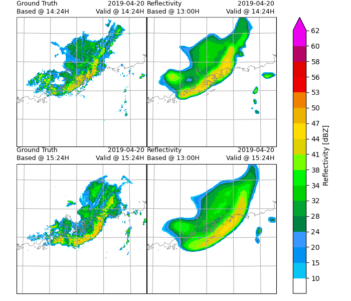
Total running time of the script: ( 0 minutes 49.220 seconds)