Note
Click here to download the full example code
SAFNWC data
This example demonstrates how to read SAFNWC data files.
Definitions
Import all required modules and methods:
# Python package to allow system command line functions
import os
# Python package for typing information
from typing import Tuple
# Python package for time calculations
import pandas as pd
# Python package for numerical calculations
import numpy as np
# Python package for projection
import cartopy.crs as ccrs
# Python package for land/sea features
import cartopy.feature as cfeature
# Python package for reading map shape file
import cartopy.io.shapereader as shpreader
# Python package for creating plots
from matplotlib import pyplot as plt
# Python package for colorbars
from matplotlib.colors import BoundaryNorm, ListedColormap

# swirlspy h8 parser function
import swirlspy.sat.safnwc as SAFNWC
# directory constants
from swirlspy.tests.samples import DATA_DIR
from swirlspy.tests.outputs import OUTPUT_DIR

plt.switch_backend('agg')

start_time = pd.Timestamp.now()
Initialising
This section demonstrates parsing Himawari-8 data.
Step 1: Define necessary parameter.
# Define data boundary in WGS84 (latitude)
latitude_from = 30.
latitude_to = 16.
longitude_from = 105.
longitude_to = 122.

extents = (
    longitude_from, longitude_to,
    latitude_from, latitude_to
)

# Define grid size, use negative value for descending range
grid_size = (-.025, .025)
Step 2: Define data directory
# Supply data directory.
data_dir = os.path.join(DATA_DIR, "safnwc")

initialising_time = pd.Timestamp.now()
Step 3: use ct, hrw as example. Other product will use similar flow as CT.
ct_path = os.path.join(
    data_dir,
    f'S_NWC_CT_HIMA08_HKOxRSMC-NR_20211108T000000Z.nc'
)

with SAFNWC.read_ct(
    ct_path,
    top=latitude_from,
    bottom=latitude_to,
    y_step=grid_size[0],
    left=longitude_from,
    right=longitude_to,
    x_step=grid_size[1]
) as ds:
    ct = ds['ct']
    ct_pal = ds['ct_pal']
    ct_attrs = ds.attrs

hrw_grouping = [
    ("all", None)
]
hrw_path = os.path.join(
    data_dir,
    f'S_NWC_HRW_HIMA08_HKOxRSMC-BS_20211108T000000Z.nc'
)
with SAFNWC.read_hrw(
    hrw_path,
    hrw_group=hrw_grouping,
    top=latitude_from,
    bottom=latitude_to,
    y_step=grid_size[0],
    left=longitude_from,
    right=longitude_to,
    x_step=grid_size[1]) as ds:
    hrw = ds[f"hrw_{hrw_grouping[0][0]}"]
    hrw_pal = ds['hrw_pal']
    hrw_attrs = ds.attrs


# CT data
print(ct)

# HRW data
print(hrw)

safnwc_time = pd.Timestamp.now()
Out:
<xarray.DataArray 'ct' (ny: 561, nx: 681)>
array([[ 7,  7,  7, ..., 11, 11,  7],
       [ 7,  7,  7, ...,  5, 10, 11],
       [ 7,  7,  7, ...,  7, 10, 10],
       ...,
       [ 1,  1,  1, ...,  8,  8,  8],
       [ 1,  1,  1, ...,  8,  8,  8],
       [ 1,  1,  1, ...,  9,  8,  9]], dtype=uint64)
Coordinates:
  * ny       (ny) float32 30.0 29.98 29.95 29.92 29.9 ... 16.08 16.05 16.02 16.0
  * nx       (nx) float32 105.0 105.0 105.1 105.1 ... 121.9 121.9 122.0 122.0
Attributes:
    long_name:             NWC GEO CT Cloud Type
    valid_range:           [ 1 15]
    ancillary_variables:   ct_status_flag ct_conditions ct_quality ct_pal
    comment:               1:  Cloud-free land; 2:  Cloud-free sea; 3:  Snow ...
    flag_values:           [ 1  2  3  4  5  6  7  8  9 10 11 12 13 14 15]
    flag_meanings:         Cloud-free_land Cloud-free_sea Snow_over_land Sea_...
    y_step:                -0.025
    x_step:                0.025
    nominal_product_time:  2021-11-08T00:00:00Z
<xarray.DataArray 'hrw_all' (barb: 5, y: 561, x: 681)>
array([[[          nan,           nan,           nan, ...,
                   nan,           nan,           nan],
        [          nan,           nan,           nan, ...,
                   nan,           nan,           nan],
        [          nan,           nan,           nan, ...,
                   nan,           nan,           nan],
        ...,
        [          nan,           nan,           nan, ...,
                   nan,           nan,           nan],
        [          nan,           nan,           nan, ...,
                   nan,           nan,           nan],
        [          nan,           nan,           nan, ...,
         5.8132987e+00,           nan,           nan]],

       [[          nan,           nan,           nan, ...,
                   nan,           nan,           nan],
        [          nan,           nan,           nan, ...,
                   nan,           nan,           nan],
        [          nan,           nan,           nan, ...,
                   nan,           nan,           nan],
...
        [          nan,           nan,           nan, ...,
                   nan,           nan,           nan],
        [          nan,           nan,           nan, ...,
                   nan,           nan,           nan],
        [          nan,           nan,           nan, ...,
         3.9261017e+00,           nan,           nan]],

       [[          nan,           nan,           nan, ...,
                   nan,           nan,           nan],
        [          nan,           nan,           nan, ...,
                   nan,           nan,           nan],
        [          nan,           nan,           nan, ...,
                   nan,           nan,           nan],
        ...,
        [          nan,           nan,           nan, ...,
                   nan,           nan,           nan],
        [          nan,           nan,           nan, ...,
                   nan,           nan,           nan],
        [          nan,           nan,           nan, ...,
         4.2872095e+00,           nan,           nan]]], dtype=float32)
Coordinates:
  * barb     (barb) <U14 'wind_speed' 'wind_direction' 'air_pressure' 'u' 'v'
  * y        (y) float32 30.0 29.98 29.95 29.92 29.9 ... 16.08 16.05 16.02 16.0
  * x        (x) float32 105.0 105.0 105.1 105.1 ... 121.9 121.9 122.0 122.0
Generating result map
Define the color scale and format of the plots and plot using xarray.plot().
In this example, only hourly images will be plotted.
# Defining the crs
crs = ccrs.PlateCarree()
# Defining coastlines
map_shape_file = os.path.join(DATA_DIR, "shape/rsmc")
coastline = cfeature.ShapelyFeature(
list(shpreader.Reader(map_shape_file).geometries()),
ccrs.PlateCarree()
)
# Defining plotting function
def _format_axis_value(v: float):
return '%g' % (v)
def _setup_fig(
axis_x: list, axis_y: list,
time_string: str, name: str,
norm: BoundaryNorm, cmap: ListedColormap,
ticks: list, ticks_loc: list,
dpi: int,
map_shape_file: str,
ocean_color: list,
land_color: list,
invert_colorbar: bool = False
) -> Tuple[plt.Figure, plt.Axes]:
# cofig
width, height = 1920, 1080
# color mappable
mappable = plt.cm.ScalarMappable(
norm=norm,
cmap=cmap
)
mappable.set_array([])
# base_map plotting function
def plot_base(ax: plt.Axes):
ax.set_extent(extents, crs=ccrs.PlateCarree())
# coastline and province
coastline_province = cfeature.ShapelyFeature(
list(shpreader.Reader(map_shape_file).geometries()),
ccrs.PlateCarree()
)
# fake the ocean color
ax.imshow(np.tile(ocean_color, [2, 2, 1]),
origin='upper',
transform=ccrs.PlateCarree(),
extent=[-180, 180, -180, 180],
zorder=-1)
# coastline, state, color
ax.add_feature(coastline_province,
facecolor=land_color, edgecolor='none', zorder=0)
# overlay coastline, state without color
ax.add_feature(coastline_province, facecolor='none',
edgecolor='white', linewidth=0.5)
# axis_ticks plotting function
def plot_axis_ticks(ax: plt.Axes, fontsize: float):
xticks = np.arange(axis_x.min(), axis_x.max(), 10)
ax.set_xticks(xticks)
ax.set_xticklabels(
[f'{_format_axis_value(t)}W' if t <
0 else f'{_format_axis_value(t)}E' for t in xticks],
fontsize=fontsize
)
yticks = np.arange(axis_y.min(), axis_y.max(), 10)
ax.set_yticks(yticks)
ax.set_yticklabels(
[f'{_format_axis_value(t)}S' if t <
0 else f'{_format_axis_value(t)}N' for t in yticks],
fontsize=fontsize
)
##############################################################################
# Step 3: Plotting the swirls-radar-advection, nwp-bias-corrected, blended 3 hours ahead
#
fig: plt.Figure = plt.figure(
figsize=(width / dpi, height / dpi)
)
gs = plt.GridSpec(
1, 1, figure=fig,
# wspace=0, hspace=0, top=0.95, bottom=0.05, left=0.27, right=0.845
wspace=0, hspace=0, top=0.95, bottom=0.05, left=0.18, right=0.845
)
ax: plt.Axes = fig.add_subplot(
gs[0, 0],
projection=ccrs.PlateCarree()
)
fig.subplots_adjust(left=.02, right=.98, bottom=.02,
top=.98, wspace=.0, hspace=.0)
# plot base map
plot_base(ax)
# axis ticks
fontsize = height * 0.01
plot_axis_ticks(ax, fontsize)
# title
fontsize = height * 0.01
ax.set_title(
time_string,
fontsize=fontsize,
loc='left',
color="white"
)
ax.set_title(
name,
fontsize=fontsize,
loc='right',
color="white"
)
fontsize = height * 0.009
cbar_ax = fig.add_axes([0.85, 0.1, 0.01, 0.8])
cbar_ax.tick_params(labelsize=fontsize)
cbar = fig.colorbar(mappable, cax=cbar_ax, extend='neither')
cbar.set_ticks(ticks_loc)
cbar.set_ticklabels(ticks)
if invert_colorbar:
cbar.ax.invert_yaxis()
fig.patch.set_facecolor('#000000')
fig.set_edgecolor('#FFFFFF')
for x in [ax, cbar_ax]:
x.tick_params(color='#FFFFFF', labelcolor='#FFFFFF')
for spine in ax.spines.values():
spine.set_edgecolor('#FFFFFF')
cbar.outline.set_edgecolor('#FFFFFF')
return fig, ax
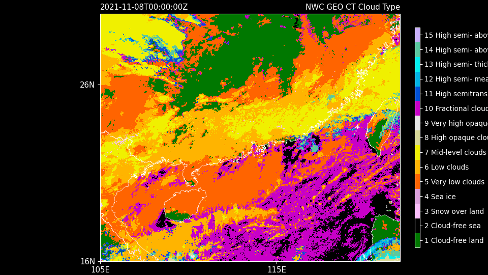
# plot CT product
# extract color palette information
k = 16
colors = (ct_pal.data[1:k, :]) / 255.0
levels = np.linspace(1, k, k)
level_ticks = [
"Cloud-free land", "Cloud-free sea", "Snow over land", "Sea ice", "Very low clouds",
"Low clouds", "Mid-level clouds", "High opaque clouds", "Very high opaque clouds", "Fractional clouds",
"High semitransparent thin", "High semi- meanly thick", "High semi- thick", "High semi- above low/med", "High semi- above snow/ice"
]
level_ticks = [f'{i + 1} {l}' for i, l in enumerate(level_ticks)]
level_ticks_loc = [
l + (levels[i + 1] - l if i < k - 1 else l - levels[i - 1]) / 2
for i, l in enumerate(levels)
]
# color map
cmap = ListedColormap(colors)
# boundary
norm = BoundaryNorm(levels, ncolors=cmap.N, clip=True)
# axis
dim_y, dim_x = ct.dims[-2:]
axis_x = ct.coords[dim_x].values
axis_y = ct.coords[dim_y].values
# setup base figure
fig, ax = _setup_fig(
axis_x, axis_y,
ct_attrs['nominal_product_time'],
ct_attrs['long_name'],
norm, cmap,
level_ticks, level_ticks_loc,
200,
map_shape_file,
ocean_color=colors[1],
land_color=colors[0]
)
# plot actual data on map
ct.where(ct >= 2).plot(
ax=ax,
cmap=cmap,
norm=norm,
add_colorbar=False,
add_labels=False
)
fig.savefig(
os.path.join(OUTPUT_DIR, "safnwc_ct.png"),
dpi=200,
bbox_inches="tight",
pad_inches=0.1,
facecolor=fig.get_facecolor(),
edgecolor='none'
)
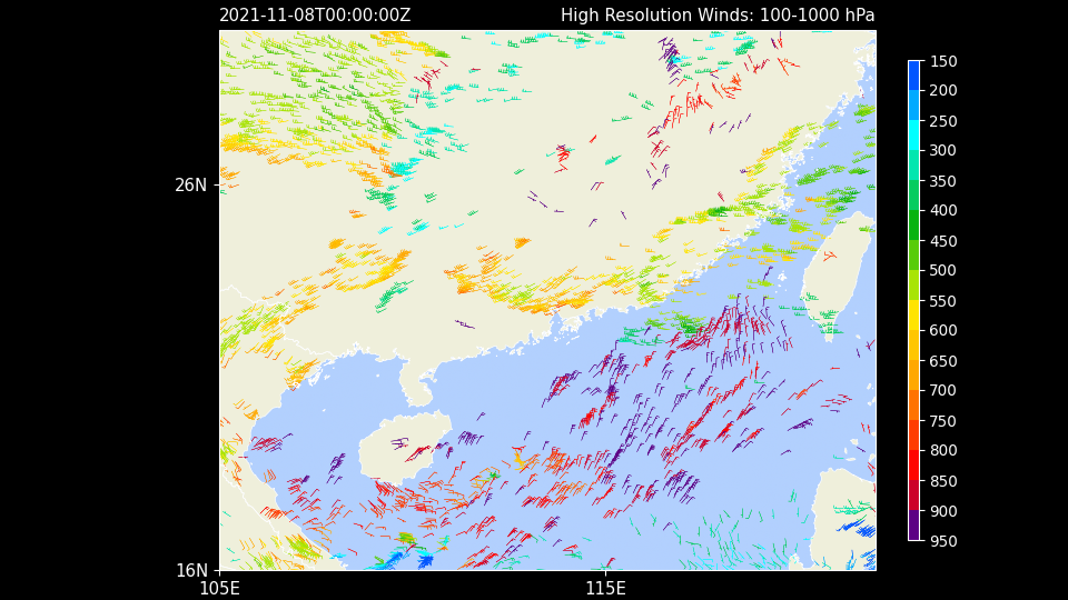
# plot HRW product
# axis
dim_y, dim_x = hrw.dims[-2:]
axis_x = hrw.coords[dim_x].values
axis_y = hrw.coords[dim_y].values
# extract necessary data
barb = list(hrw.coords['barb'].values)
ap_idx = barb.index('air_pressure')
u_idx = barb.index('u')
v_idx = barb.index('v')
# filter non null data
y = np.repeat(axis_y, hrw.shape[2]).reshape(hrw.shape[1:])
x = np.tile(axis_x, hrw.shape[1]).reshape(hrw.shape[1:])
idx = np.isnan(hrw[ap_idx, :, :])
hrw_data = np.concatenate((hrw, [y], [x]))[:, ~idx]
# filter non null data
x = hrw_data[-1, :]
y = hrw_data[-2, :]
u = hrw_data[u_idx, :]
v = hrw_data[v_idx, :]
flip_barb = y < 0
air_pressure = hrw_data[ap_idx, :] / 100
# extract color palette information
levels = [150, 200, 250, 300, 350, 400, 450, 500,
550, 600, 650, 700, 750, 800, 850, 900, 950]
colors = (hrw_pal.data[11:199:11]) / 255.0
# color map
cmap = ListedColormap(colors)
# boundary
norm = BoundaryNorm(levels, ncolors=cmap.N, clip=True)
fig, ax = _setup_fig(
axis_x, axis_y,
hrw_attrs['nominal_product_time'],
f"High Resolution Winds: 100-1000 hPa",
norm, cmap,
levels, levels,
200,
map_shape_file,
ocean_color=np.array([178, 208, 254], dtype=np.uint8) / 255.,
land_color=cfeature.COLORS['land'],
invert_colorbar=True
)
ax = ax.barbs(
x, y, u, v, air_pressure,
cmap=cmap, norm=norm,
sizes={'spacing': 0.2, 'width': 0.15, 'height': 0.3, 'emptybarb': 0.0},
length=3.5, linewidth=0.25,
flip_barb=flip_barb,
pivot='middle',
barb_increments={'half': 2.5722810989, 'full': 5.1445621978, 'flag': 25.7228109888}
)
fig.savefig(
os.path.join(OUTPUT_DIR, "safnwc_hrw.png"),
dpi=200,
bbox_inches="tight",
pad_inches=0.1,
facecolor=fig.get_facecolor(),
edgecolor='none'
)
safnwc_image_time = pd.Timestamp.now()
Checking run time of each component
print(f"Start time: {start_time}")
print(f"Initialising time: {initialising_time}")
print(f"SAFNWC data parsing time: {safnwc_time}")
print(f"Plotting safnwc image time: {safnwc_image_time}")

print(f"Time to initialise: {initialising_time - start_time}")
print(f"Time to run data parsing: {safnwc_time - initialising_time}")
print(f"Time to plot data images: {safnwc_image_time - safnwc_time}")
Out:
Start time: 2025-10-11 04:31:22.143769
Initialising time: 2025-10-11 04:31:22.144578
SAFNWC data parsing time: 2025-10-11 04:31:26.592182
Plotting safnwc image time: 2025-10-11 04:31:31.811159
Time to initialise: 0 days 00:00:00.000809
Time to run data parsing: 0 days 00:00:04.447604
Time to plot data images: 0 days 00:00:05.218977
Total running time of the script: ( 0 minutes 9.663 seconds)