Note
Click here to download the full example code
SPROG (Hong Kong)
This example demonstrates how to use SPROG to forecast rainfall up to three hours, using rain guage and radar data from Hong Kong.
Definitions
Import all required modules and methods:
# Python package to allow system command line functions
import os
# Python package to manage warning message
import warnings
# Python package for time calculations
import pandas as pd
# Python package for numerical calculations
import numpy as np
# Python package for xarrays to read and handle netcdf data
import xarray as xr
# Python package for text formatting
import textwrap
# Python package for projection description
from pyresample import get_area_def
# Python package for projection
import cartopy.crs as ccrs
# Python package for land/sea features
import cartopy.feature as cfeature
# Python package for reading map shape file
import cartopy.io.shapereader as shpreader
# Python package for creating plots
from matplotlib import pyplot as plt
# Python package for output grid format
from matplotlib.gridspec import GridSpec
# Python package for colorbars
from matplotlib.colors import BoundaryNorm, ListedColormap
from matplotlib.cm import ScalarMappable

# swirlspy data parser function
from swirlspy.rad.iris import read_iris_grid
# swirlspy test data source locat utils function
from swirlspy.qpe.utils import timestamps_ending, locate_file
# swirlspy regrid function
from swirlspy.core.resample import grid_resample
# swirlspy standardize data function
from swirlspy.utils import FrameType, standardize_attr, conversion
# swirlspy pysteps integrated package
from swirlspy.qpf import sprog, dense_lucaskanade
# directory constants
from swirlspy.tests.samples import DATA_DIR
from swirlspy.tests.outputs import OUTPUT_DIR

warnings.filterwarnings("ignore")
Define working directory and nowcast parameters:
radar_dir = os.path.abspath(
    os.path.join(DATA_DIR, 'iris/ppi')
)

# Set nowcast parameters
n_timesteps = int(3 * 60 / 6)  # 3 hours, each timestamp is 6 minutes
Define the user grid:
area_id = "hk1980_250km"
description = (
    "A 250 m resolution rectangular grid centred at HKO and extending"
    "to 250 km in each direction in HK1980 easting/northing coordinates"
)
proj_id = 'hk1980'
projection = (
    '+proj=tmerc +lat_0=22.31213333333334 '
    '+lon_0=114.1785555555556 +k=1 +x_0=836694.05 '
    '+y_0=819069.8 +ellps=intl +towgs84=-162.619,-276.959,'
    '-161.764,0.067753,-2.24365,-1.15883,-1.09425 +units=m +no_defs'
)
x_size = 500
y_size = 500
area_extent = (587000, 569000, 1087000, 1069000)
area_def_tgt = get_area_def(
    area_id, description, proj_id, projection, x_size, y_size, area_extent
)
Define the base map:
# Load the shape of Hong Kong
map_shape_file = os.path.abspath(os.path.join(
    DATA_DIR,
    'shape/hk'
))

# coastline and province
map_with_province = cfeature.ShapelyFeature(
    list(shpreader.Reader(map_shape_file).geometries()),
    ccrs.PlateCarree()
)


# define the plot function
def plot_base(ax: plt.Axes, extents: list, crs: ccrs.Projection):
    ax.set_extent(extents, crs=crs)
    # fake the ocean color
    ax.imshow(
        np.tile(np.array([[[178, 208, 254]]], dtype=np.uint8), [2, 2, 1]),
        origin='upper', transform=ccrs.PlateCarree(),
        extent=[-180, 180, -180, 180], zorder=-1
    )
    # coastline, province and state, color
    ax.add_feature(
        map_with_province, facecolor=cfeature.COLORS['land'],
        edgecolor='none', zorder=0
    )
    # overlay coastline, province and state without color
    ax.add_feature(
        map_with_province, facecolor='none', edgecolor='gray', linewidth=0.5
    )
    ax.set_title('')
Log the start time for reference:
start_time = pd.Timestamp.now()
Loading Radar Data
# Specify the basetime
basetime = pd.Timestamp('201902190800')

# Generate a list of timestamps of the radar data files
located_files = []
radar_ts = timestamps_ending(
    basetime,
    duration=pd.Timedelta(minutes=60),
    exclude_end=False
)
for timestamp in radar_ts:
    located_files.append(locate_file(radar_dir, timestamp))

# Read in the radar data
reflectivity_list = []  # stores reflec from read_iris_grid()
for filename in located_files:
    reflec = read_iris_grid(filename)
    reflectivity_list.append(reflec)

# Reproject the radar data to the user-defined grid
area_def_src = reflectivity_list[0].attrs['area_def']
reproj_reflectivity_list = []
for reflec in reflectivity_list:
    reproj_reflec = grid_resample(
        reflec, area_def_src, area_def_tgt,
        coord_label=['x', 'y']
    )
    reproj_reflectivity_list.append(reproj_reflec)

# Standardize reflectivity xarrays
raw_frames = xr.concat(reproj_reflectivity_list,
                       dim='time').sortby(['y'], ascending=False)
standardize_attr(raw_frames, frame_type=FrameType.dBZ)

# Transform from reflecitiy to rainfall rate
frames = conversion.to_rainfall_rate(raw_frames, True, a=58.53, b=1.56)

# Set the fill value
frames.attrs['zero_value'] = -15.0

# Apply threshold to -10dBR i.e. 0.1mm/h
threshold = -10.0
frames.values[frames.values < threshold] = frames.attrs['zero_value']

# Set missing values with the fill value
frames.values[~np.isfinite(frames.values)] = frames.attrs['zero_value']


# Log the time for record
initialising_time = pd.Timestamp.now()
Running Lucas Kanade Optical flow and S-PROG
# Estimate the motion field
motion = dense_lucaskanade(frames)

motion_time = pd.Timestamp.now()

# Generate forecast rainrate field
forcast_frames = sprog(
    frames,
    motion,
    n_timesteps,
    n_cascade_levels=8,
    R_thr=threshold,
    decomp_method="fft",
    bandpass_filter_method="gaussian",
    probmatching_method="mean",
)

sprog_time = pd.Timestamp.now()
Out:
Pysteps configuration file found at: /builds/com-swirls/swirlspy/.cache/conda/envs/swirlspy/lib/python3.6/site-packages/pysteps/pystepsrc

Computing S-PROG nowcast:
-------------------------

Inputs:
-------
input dimensions: 500x500

Methods:
--------
extrapolation:          semilagrangian
bandpass filter:        gaussian
decomposition:          fft
conditional statistics: no
probability matching:   mean
FFT method:             numpy
domain:                 spatial

Parameters:
-----------
number of time steps:     30
parallel threads:         1
number of cascade levels: 8
order of the AR(p) model: 2
precip. intensity threshold: -10
************************************************
* Correlation coefficients for cascade levels: *
************************************************
-----------------------------------------
| Level |     Lag-1     |     Lag-2     |
-----------------------------------------
| 1     | 0.998920      | 0.996649      |
-----------------------------------------
| 2     | 0.998260      | 0.995759      |
-----------------------------------------
| 3     | 0.991719      | 0.979920      |
-----------------------------------------
| 4     | 0.968905      | 0.917719      |
-----------------------------------------
| 5     | 0.855422      | 0.667819      |
-----------------------------------------
| 6     | 0.493524      | 0.215498      |
-----------------------------------------
| 7     | 0.084985      | 0.006179      |
-----------------------------------------
| 8     | -0.003395     | 0.002382      |
-----------------------------------------
****************************************
* AR(p) parameters for cascade levels: *
****************************************
------------------------------------------------------
| Level |    Phi-1     |    Phi-2     |    Phi-0     |
------------------------------------------------------
| 1     | 1.550586     | -0.552262    | 0.038733     |
------------------------------------------------------
| 2     | 1.217599     | -0.219721    | 0.057523     |
------------------------------------------------------
| 3     | 1.207339     | -0.217421    | 0.125356     |
------------------------------------------------------
| 4     | 1.302167     | -0.343957    | 0.232335     |
------------------------------------------------------
| 5     | 1.059279     | -0.238312    | 0.503009     |
------------------------------------------------------
| 6     | 0.511836     | -0.037105    | 0.869133     |
------------------------------------------------------
| 7     | 0.085074     | -0.001051    | 0.996382     |
------------------------------------------------------
| 8     | -0.003387    | 0.002370     | 0.999991     |
------------------------------------------------------
Starting nowcast computation.
Computing nowcast for time step 1... done.
Computing nowcast for time step 2... done.
Computing nowcast for time step 3... done.
Computing nowcast for time step 4... done.
Computing nowcast for time step 5... done.
Computing nowcast for time step 6... done.
Computing nowcast for time step 7... done.
Computing nowcast for time step 8... done.
Computing nowcast for time step 9... done.
Computing nowcast for time step 10... done.
Computing nowcast for time step 11... done.
Computing nowcast for time step 12... done.
Computing nowcast for time step 13... done.
Computing nowcast for time step 14... done.
Computing nowcast for time step 15... done.
Computing nowcast for time step 16... done.
Computing nowcast for time step 17... done.
Computing nowcast for time step 18... done.
Computing nowcast for time step 19... done.
Computing nowcast for time step 20... done.
Computing nowcast for time step 21... done.
Computing nowcast for time step 22... done.
Computing nowcast for time step 23... done.
Computing nowcast for time step 24... done.
Computing nowcast for time step 25... done.
Computing nowcast for time step 26... done.
Computing nowcast for time step 27... done.
Computing nowcast for time step 28... done.
Computing nowcast for time step 29... done.
Computing nowcast for time step 30... done.
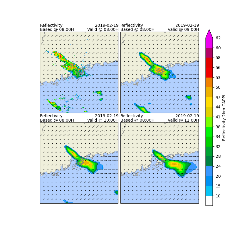
Generating radar reflectivity maps
Define the color scale and format of the plot.
# Defining colour scale and  format.
levels = [
    -32768, 10, 15, 20, 24, 28, 32, 34, 38, 41, 44, 47, 50, 53, 56, 58, 60, 62
]
cmap = ListedColormap([
    '#FFFFFF00', '#08C5F5', '#0091F3', '#3898FF', '#008243', '#00A433',
    '#00D100', '#01F508', '#77FF00', '#E0D100', '#FFDC01', '#EEB200',
    '#F08100', '#F00101', '#E20200', '#B40466', '#ED02F0'
])

norm = BoundaryNorm(levels, ncolors=cmap.N, clip=True)

mappable = ScalarMappable(cmap=cmap, norm=norm)
mappable.set_array([])

# Defining the crs
crs = area_def_tgt.to_cartopy_crs()

# Defining area
x = frames.coords['x'].values
y = frames.coords['y'].values
x_d = x[1] - x[0]
y_d = y[1] - y[0]
extents = [x[0], y[0], x[-1], y[-1]]

# Generating a time steps for every hour
time_steps = [
    basetime + pd.Timedelta(minutes=6*i)
    for i in range(n_timesteps + 1) if i % 10 == 0
]

ref_frames = conversion.to_reflectivity(forcast_frames, True)
ref_frames.data[ref_frames.data < 0.1] = np.nan
ref_frames = xr.concat([raw_frames[:-1, ...], ref_frames], dim='time')
ref_frames.attrs['values_name'] = 'Reflectivity 2km CAPPI'
standardize_attr(ref_frames)

qx = motion.coords['x'].values[::5]
qy = motion.coords['y'].values[::5]
qu = motion.values[0, ::5, ::5]
qv = motion.values[1, ::5, ::5]

fig: plt.Figure = plt.figure(figsize=(8, 8), frameon=False)
gs = GridSpec(
    2, 2, figure=fig, wspace=0.03, hspace=-0.25, top=0.95,
    bottom=0.05, left=0.17, right=0.845
)

for i, t in enumerate(time_steps):
    row = i // 2
    col = i % 2
    ax = fig.add_subplot(gs[row, col], projection=crs)

    # plot base map
    plot_base(ax, extents, crs)

    # plot reflectivity
    frame = ref_frames.sel(time=t)
    im = ax.imshow(frame.values, cmap=cmap, norm=norm, interpolation='nearest',
                   extent=extents)

    # plot motion vector
    ax.quiver(qx, qy, qu, qv, pivot='mid', regrid_shape=20)

    ax.text(
        extents[0],
        extents[1],
        textwrap.dedent(
            """
            Reflectivity
            Based @ {baseTime}
            """
        ).format(
            baseTime=basetime.strftime('%H:%MH')
        ).strip(),
        fontsize=10,
        va='bottom',
        ha='left',
        linespacing=1
    )
    ax.text(
        extents[2] - (extents[2] - extents[0]) * 0.03,
        extents[1],
        textwrap.dedent(
            """
            {validDate}
            Valid @ {validTime}
            """
        ).format(
            validDate=basetime.strftime('%Y-%m-%d'),
            validTime=t.strftime('%H:%MH')
        ).strip(),
        fontsize=10,
        va='bottom',
        ha='right',
        linespacing=1
    )

cbar_ax = fig.add_axes([0.875, 0.125, 0.03, 0.75])
cbar = fig.colorbar(
    mappable, cax=cbar_ax, ticks=levels[1:], extend='max', format='%.3g')
cbar.ax.set_ylabel(ref_frames.attrs['values_name'], rotation=90)

fig.savefig(
    os.path.join(
        OUTPUT_DIR,
        "sprog-reflectivity.png"
    ),
    bbox_inches='tight'
)

radar_image_time = pd.Timestamp.now()
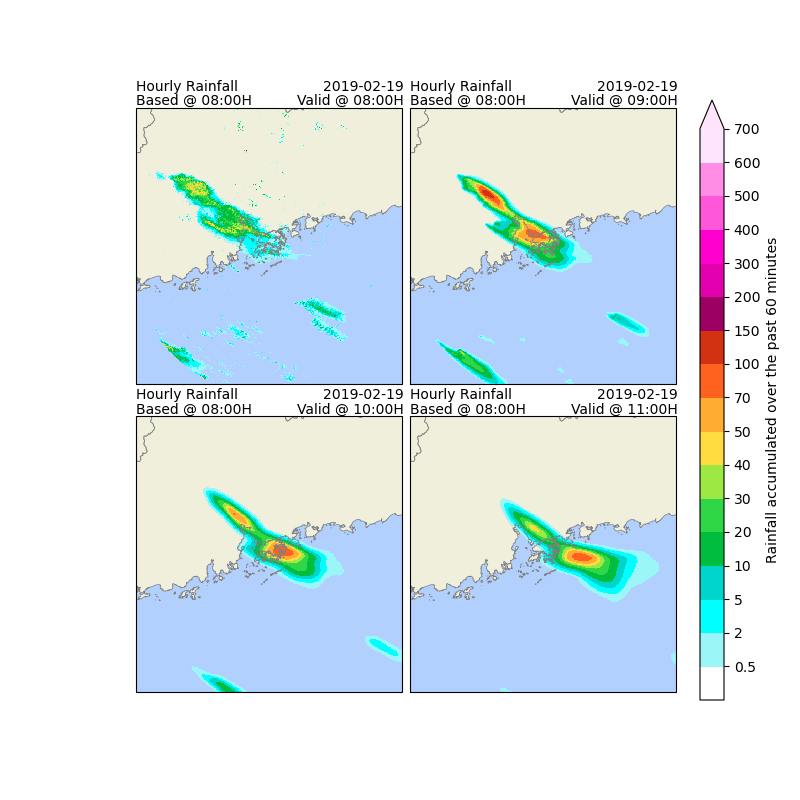
Accumulating hourly rainfall for 3-hour forecast
Hourly accumulated rainfall is calculated every 30 minutes, the first endtime is the basetime i.e. T+30min.
# Optional, convert to rainfall depth
rf_frames = conversion.to_rainfall_depth(ref_frames, a=58.53, b=1.56)

# Compute hourly accumulated rainfall every 60 minutes.
acc_rf_frames = conversion.acc_rainfall_depth(
    rf_frames,
    basetime,
    basetime + pd.Timedelta(hours=3),
    pd.Timedelta(minutes=60)
)


# Replace zero value with NaN
acc_rf_frames.data[acc_rf_frames.data <=
                   acc_rf_frames.attrs['zero_value']] = np.nan

acc_time = pd.Timestamp.now()
Generating radar reflectivity maps
# Defining colour scale and  format.
levels = [
    0, 0.5, 2, 5, 10, 20,
    30, 40, 50, 70, 100, 150,
    200, 300, 400, 500, 600, 700
]
cmap = ListedColormap([
    '#ffffff00', '#9bf7f7', '#00ffff', '#00d5cc', '#00bd3d', '#2fd646',
    '#9de843', '#ffdd41', '#ffac33', '#ff621e', '#d23211', '#9d0063',
    '#e300ae', '#ff00ce', '#ff57da', '#ff8de6', '#ffe4fd'
])

norm = BoundaryNorm(levels, ncolors=cmap.N, clip=True)

mappable = ScalarMappable(cmap=cmap, norm=norm)
mappable.set_array([])

fig: plt.Figure = plt.figure(figsize=(8, 8), frameon=False)
gs = GridSpec(
    2, 2, figure=fig, wspace=0.03, hspace=-0.25, top=0.95,
    bottom=0.05, left=0.17, right=0.845
)

for i, t in enumerate(acc_rf_frames.coords['time'].values):
    row = i // 2
    col = i % 2
    ax = fig.add_subplot(gs[row, col], projection=crs)

    # plot base map
    plot_base(ax, extents, crs)

    # plot accumulated rainfall depth
    t = pd.Timestamp(t)
    frame = acc_rf_frames.sel(time=t)
    im = ax.imshow(frame.values, cmap=cmap, norm=norm, interpolation='nearest',
                   extent=extents)

    ax.text(
        extents[0],
        extents[1],
        textwrap.dedent(
            """
            Hourly Rainfall
            Based @ {baseTime}
            """
        ).format(
            baseTime=basetime.strftime('%H:%MH')
        ).strip(),
        fontsize=10,
        va='bottom',
        ha='left',
        linespacing=1
    )
    ax.text(
        extents[2] - (extents[2] - extents[0]) * 0.03,
        extents[1],
        textwrap.dedent(
            """
            {validDate}
            Valid @ {validTime}
            """
        ).format(
            validDate=basetime.strftime('%Y-%m-%d'),
            validTime=t.strftime('%H:%MH')
        ).strip(),
        fontsize=10,
        va='bottom',
        ha='right',
        linespacing=1
    )

cbar_ax = fig.add_axes([0.875, 0.125, 0.03, 0.75])
cbar = fig.colorbar(
    mappable, cax=cbar_ax, ticks=levels[1:], extend='max', format='%.3g')
cbar.ax.set_ylabel(acc_rf_frames.attrs['values_name'], rotation=90)

fig.savefig(
    os.path.join(
        OUTPUT_DIR,
        "sprog-rainfall.png"
    ),
    bbox_inches='tight'
)

ptime = pd.Timestamp.now()
Checking run time of each component
print(f"Start time: {start_time}")
print(f"Initialising time: {initialising_time}")
print(f"Motion field time: {motion_time}")
print(f"S-PROG time: {sprog_time}")
print(f"Plotting radar image time: {radar_image_time}")
print(f"Accumulating rainfall time: {acc_time}")
print(f"Plotting rainfall maps: {ptime}")

print(f"Time to initialise: {initialising_time - start_time}")
print(f"Time to run motion field: {motion_time - initialising_time}")
print(f"Time to perform S-PROG: {sprog_time - motion_time}")
print(f"Time to plot radar image: {radar_image_time - sprog_time}")
print(f"Time to accumulate rainfall: {acc_time - radar_image_time}")
print(f"Time to plot rainfall maps: {ptime - acc_time}")

print(f"Total: {ptime - start_time}")
Out:
Start time: 2025-10-11 04:44:28.464614
Initialising time: 2025-10-11 04:44:34.359015
Motion field time: 2025-10-11 04:44:36.473976
S-PROG time: 2025-10-11 04:44:41.382591
Plotting radar image time: 2025-10-11 04:44:52.709358
Accumulating rainfall time: 2025-10-11 04:44:53.500320
Plotting rainfall maps: 2025-10-11 04:45:02.894817
Time to initialise: 0 days 00:00:05.894401
Time to run motion field: 0 days 00:00:02.114961
Time to perform S-PROG: 0 days 00:00:04.908615
Time to plot radar image: 0 days 00:00:11.326767
Time to accumulate rainfall: 0 days 00:00:00.790962
Time to plot rainfall maps: 0 days 00:00:09.394497
Total: 0 days 00:00:34.430203
Total running time of the script: ( 0 minutes 34.030 seconds)